Volume 33, Issue 1: Paper 6
The Minimum Wage and its Impact on Employment
Joshua Hutson, Furman University
Debates surrounding minimum wage laws have permeated a good portion of public discourse in recent years. The United States Congress has not raised the federal minimum wage since 2009, almost 15 years ago. Many argue that the federal minimum wage is not enough to live on and protest to raise it. On the other side of the argument, people contend that a minimum wage increase would lead to a decrease in employment among low-income workers since companies would fire some of their unskilled laborers to offset their increased labor costs. This project aims to measure how the minimum wage impacts employment numbers using data from every continental state in the United States over the past 30 years. Assessing the risks associated with raising the minimum wage can inform decisions regarding minimum wage policy.
Until recently, the minimum wage in most states and the national minimum wage did not significantly differ from each other. However, since 2000 over half of US states have adopted new minimum wage laws, which presents the opportunity to study the minimum wage’s impact on labor markets at the national level. The variety in policy among states that are close to each other allows for the utilization of cross border analysis to determine if the minimum wage has an impact on employment within the fast-food industry and the extent of that impact. The experiments and regression models defined in this paper present no compelling evidence that the minimum wage has any impact on employment numbers.
II. BEHIND THE CURTAIN: THE THEORY OF COMPETITIVE LABOR MARKETS
In theory, the competitive labor market follows the laws of supply and demand, which state as the price for a commodity increases, the quantity supplied will increase and the quantity demanded will decrease, holding all else equal. In this market, the commodity is labor. If wages are set too low, plenty of demand for labor will exist, but very few people will be willing to supply their labor at that price point, resulting in a shortage of workers. When firms recognize that they cannot hire enough people to meet their demand, they will begin to increase their wages. If wages are set too high, the number of people willing to supply their labor will exceed the demand for labor, resulting in a surplus of workers. Firms will recognize that they can offer a lower price for labor and lower their wages for the next hiring cycle.
The minimum wage acts as a price floor in the competitive labor market, which can either be binding or non-binding. A non-binding minimum wage will not impact a given labor market, but a binding minimum wage according to theory will decrease the quantity of work demanded, as displayed in Figure 1. However, the extent of that decrease depends on market elasticity. If the demand curve is inelastic, then the quantity demanded does not change much at different price levels. If the curve is elastic, then the quantity demanded changes more at each price point.
Every labor market is different, and the minimum wage is non-binding for most of them. For the study to be informative, labor markets where the minimum wage is binding must be selected. Thus, the fast-food industry was chosen, not only because such jobs usually pay the minimum wage, but also because fast food is widespread in the United States. Counties also have different fast food labor markets, and some might have more inelastic curves than others. Fixed effects are incorporated into the coming empirical models to control for all time-constant differences in labor markets.
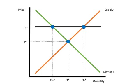
Figure 1: Binding Price Floor in a Competitive Labor Market
III. EMPIRICAL DEBATE
Empirical studies of the minimum wage provide conflicting results, which do not always match theory. David Card and Alan B. Krueger conducted an experiment with New Jersey and Pennsylvania fast food restaurants in 1992 when New Jersey raised its minimum wage and Pennsylvania did not. They found that there was no significant decrease in employment when the minimum wage changed but rather a significant increase (Card and Krueger 1993). The study sparked some controversy, prompting two other researchers to publish a response. David Neumark and William Wascher claimed that Card and Krueger’s data was faulty since they used telephone survey data to get their employment rates. These two researchers instead used payroll data, which led them to the conclusion that employment decreased when the minimum wage increased (Neumark and Wascher 2000). However, Card and Krueger wrote a reply where they reaffirmed their original findings using data from the Bureau of Labor Statistics (Card and Krueger 2000).
IV. METHODOLOGY
The following experimental design uses a difference in difference model to explain the impact of the minimum wage on employment in the fast-food industry using counties on the borders of neighboring states as control and treatment groups. The employment data comes from the Bureau of Labor Statistics Quarterly Census of Employment and Wages (“Quarterly Census of Employment and Wage 1990-2023”), restricted to limited-service restaurants in the private sector for every county in the United States. Counties that were not on the border between the two states were removed. When one state increases its minimum wage and its neighbor does not, the fast-food employment is recorded for the border counties in the year before the increase and the year after the increase. The treatment group consists of counties in the state with the minimum wage increase, and the control group consists of counties in the state where the minimum wage was constant. Figure 2 displays the experimental design at the experiment level, and Figure 3 displays all the counties in the data set.
Dube, Lester, and Reich (2010) conducted a similar analysis to the one proposed above. They also used the Quarterly Census of Employment and Wage to conduct cross border analysis, but only from 1990 to 2006 (Dube, Lester, Reich 2010). This paper adds to the existing work by including years after 2006. For example, Florida tied their minimum wage to inflation in 2006, meaning every year after 2006, more data on the impact of the minimum wage on the Florida-Georgia and Florida-Alabama border can be included in the data set. Some borders also only have experiments past 2006. The North Carolina-South Carolina, North Carolina-Tennessee, North Dakota-South Dakota, North Dakota-Wyoming, South Dakota-Nebraska, South Dakota-Wyoming, and Nebraska-Kansas borders are all not represented in Dube, Lester, and Reich’s data set because their minimum wage laws were the same until after 2006. The data in this paper’s experiments includes these border experiments. Dube Lester and Reich (2010) include full and limited-service restaurants in their data set. This experiment only uses limited-service restaurants to make the research more comparable to Card, Krueger, Neumark, and Wascher’s previous work since they only considered fast food restaurants, all of which are limited service (Card and Krueger 1993; Neumark and Wascher 2000; Card and Krueger 2000).
Several states tied their minimum wage policy to CPI, meaning they increased their minimum wage based on inflation from the previous year. Counties in those experiments are counted twice, once as a pre-minimum wage instance in one experiment and then again as a post-minimum wage instance in another experiment. For example, Florida adopted a CPI-adjusted minimum wage policy following the federal minimum wage increase in 2008 while its neighboring states, Alabama and Georgia, adopt the federal minimum wage. In the data set, the counties on the Florida-Georgia and the Florida-Alabama border are repeated twice per year from 2010, the year after the national government raised the national minimum wage, to 2021, the penultimate year in the data set. One instance represents the fast-food employment in the county before the next minimum wage increase and one represents the fast-food employment in the county after the last minimum wage increase. Other counties are also counted twice as a part of two separate experiments because they are on the border of multiple states.
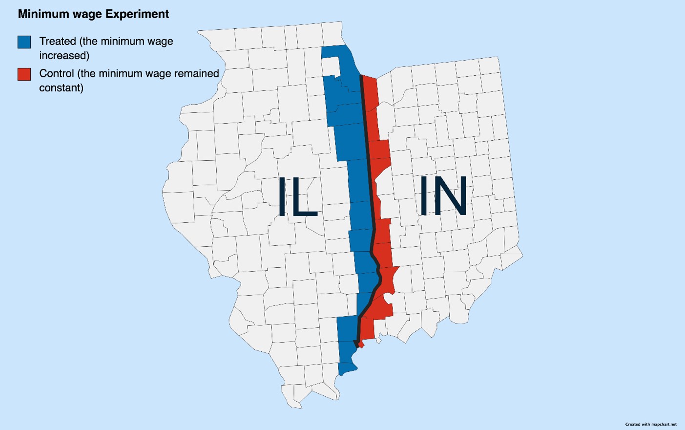
Figure 2: Minimum Wage Experiment Example
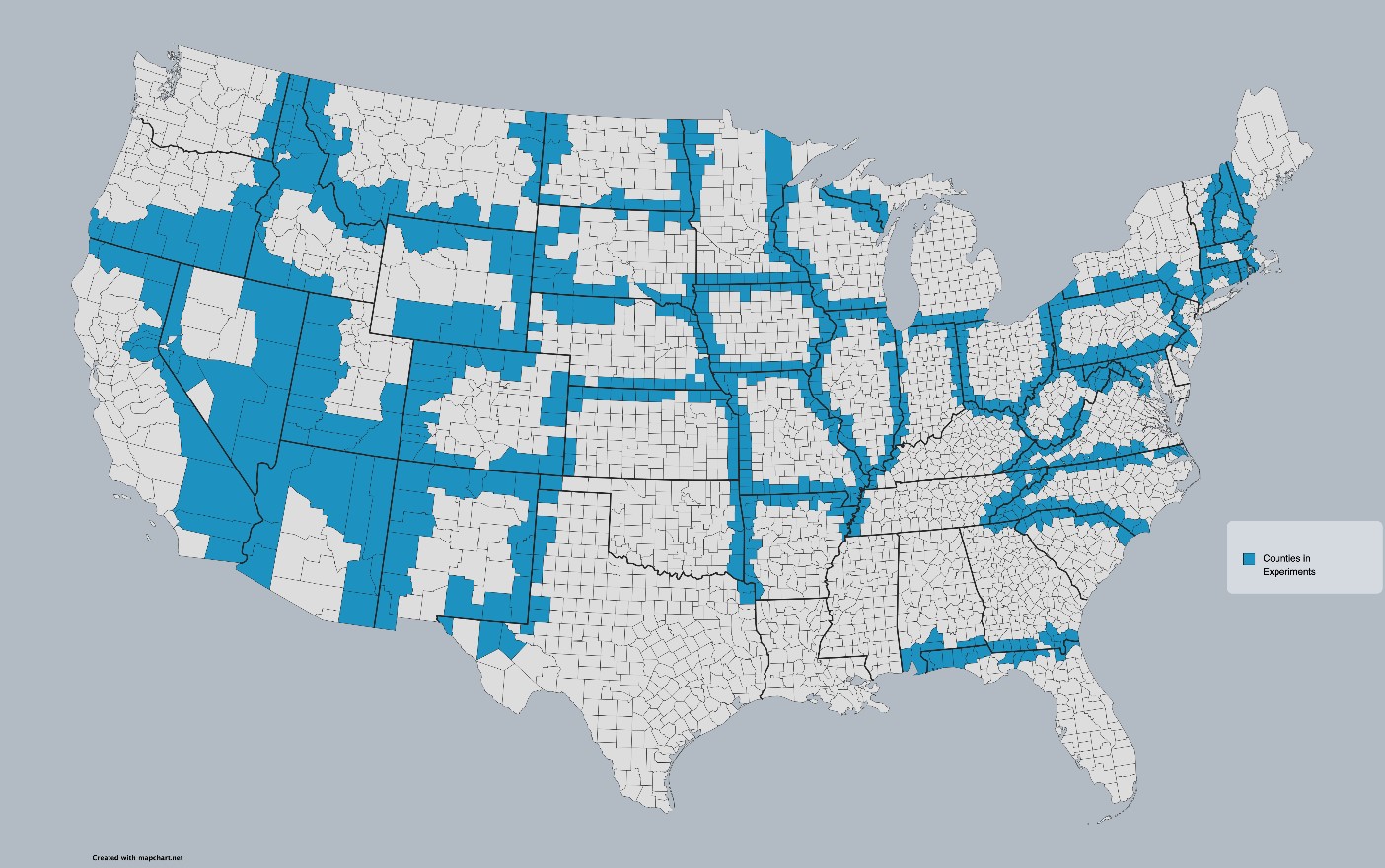
Figure 3: All Counties in Experiments
This paper’s methodology mimics that of Card and Kruger’s original study with a few changes. Card and Krueger called a random sample of 473 restaurants in New Jersey and Pennsylvania in 1991 and 1992 and recorded establishment-level data about prices, wages, benefits, location, chain name, and employment (Card and Krueger 1993). The coming analysis uses employment data from the Bureau of Labor Statistics, the same source Card and Krueger used to supplement their data in their second paper (Card and Krueger 2000). The data from the Bureau of Labor Statistics is not as specific as Card and Krueger’s but is more widely applicable. They looked at two states and compared the data they collected before and after the minimum wage took effect. In contrast, this study compares employment data for 45 states over 30 years. Although this study’s data sacrifices the specificity of Card and Krueger’s data, it gains generality and scope. The Bureau of Labor Statistics does not publicly release data about the price of fast food or employee benefits, but they do release employment numbers by industry at the county level. Card and Krueger could only make claims about the fast-food market in New Jersey and Pennsylvania, but these two states are not representative of all states.
Even with applicable data, studying the impact of the minimum wage is difficult. As Brown points out, wage elasticity, the effect of coverage, and hidden methods of compensation all make it difficult to establish a causal relationship between the minimum wage and employment (Brown 1988). To mitigate the effect of coverage, the data is restricted to limited-service restaurants, which are defined as any food-service restaurant where the service ends after the food has been received. These businesses include pizzerias, delis, cafes, and carry out restaurants, but most of the employers are fast food restaurants like McDonald’s, Starbucks, Arby’s, and Wendy’s. Such large corporations are subject to the Fair Labor Standards Act so uniformity of coverage is assumed, even though minimum wage laws may not apply to a portion of the smaller limited-service businesses like those that only have one location and hire only family members to work for them. Unlike with Card and Krueger’s data, hidden methods of compensation cannot directly be accounted for because the Bureau of Labor Statistics does not make that information publicly available. Instead, it must be assumed that the types of hidden compensation are similar across all the various companies, namely that employees can get discounted or free food, and that each company will similarly adjust their hidden benefits when the minimum wage increases.
Dube, Lester, and Reich also consider the possibility that in looking at contiguous borders, spill overs exist (Dube, Lester, Reich 2010). Spilling over means that county pairs are linked, and when one county increases wages or decreases employment, the other county might experience an influx of new workers which impacts their market conditions. To test for spillovers, the researchers compared the effects of the minimum wage on the border counties to the inland counties. The researchers found no statistically significant effect of spilling over when they ran their robustness tests (Dube, Lester, Reich 2010).
Finally, wage elasticity depends on counties. As such the coming models include fixed effects to absorb variations in wage elasticity. County fixed effects will control for all other time-constant entity-specific characteristics, like demographics or industry composition. The models also include year fixed effects to control for year-specific characteristics like inflation or market shocks that impacted all counties similarly. Beaudry, Green, and Sand also established a relationship between population and labor demand elasticity, so county population is explicitly accounted for in the models (Beaudry, Green, Sand 2018).
V. The Model
As previously stated, a difference-in-difference model was constructed to assess the role that minimum wage increases have on employment. Using the experimental data from 1990 to 2022 (t=1, 2,…, 33), the following empirical model was produced:
(1) EMPLOYi,t = 0 + 1 TREATEDi,t + 2 POSTi,t + 3(TREATEDi,t)(POSTi,t ) + i + t + 5 TOTALPOPi,t +i,t
Table 1: Description of Variables in Empirical Model
| Variable | Description | Measurement |
|---|---|---|
| TREATEDi,t | A variable indicating whether a data point belongs to the treated group whose minimum wage increased | 0 if the observation belongs to the control group;
1 if it belongs to the treated group |
| POSTi,t | A variable indicating whether a data point was collected before or after the minimum wage increase | 0 if the observation was collected before the minimum wage changed;
1 if it was collected after |
| TREATEDi,txPOSTi,t | The interaction between the two indicator variables | 1 if the observation was in the treated group after a minimum wage change;
0 otherwise |
| i | Describes estimated county fixed effects added into the model | A dummy variable for all but one county. |
| t | Describes estimated year fixed effects added into the model | A dummy variable for all but one year. |
| TOTALPOPi,t | The total population of county i at the start of a given year t | Number of people |
| EMPLOYi,t | The number of people employed in limited-service restaurants in county i at the beginning of year t | Number of people |
The variable TREATEDi,t will control for variations between the states that do and do not enact new minimum wage laws, since each state has different laws regarding labor. The variable POSTi,t will isolate the variation associated with whether the data was collected before or after the minimum wage increase. The variable of interest is the interaction term (TREATEDi,t)(POSTi,t ), which will explain how much of the variability in employment can be associated with the minimum wage.
Table 2: Summary Statistics for the data set
| Mean | Standard Deviation | |
|---|---|---|
| TREATEDi,t | 0.491 | 0.499 |
| POSTi,t | 0.504 | 0.500 |
| EMPLOYi,t | 1374.028 | 3421.881 |
Table 2 describes the breakdown of the data set. TREATEDi,t and POSTi,t both make up roughly 50 percent of the instances, meaning the data set contains roughly the same number of treated group instances and control group instances and roughly the same number of pre-minimum wage increase instances as post-minimum wage instances. Employment has a wide range of values, indicated by its standard deviation.
Several counties either did not have any fast-food employment or only had fast food employment for a few years. These counties add noise to the model because they add uninformative zeros to the data. All counties with no fast-food employment in any year were removed. The removed counties are represented in yellow in Figure 4. Additionally, there are other counties who had fast food employment in some years but not others. Within counties, the observations where the fast-food employment was zero both before and after the experiment were removed. These removals are represented in green in Figure 4. A revised data set that implemented those changes was created. The unchanged counties are still blue. The coming analysis runs two models on the original data and for robustness runs the remaining models on the revised data set depicted by Figure 4.
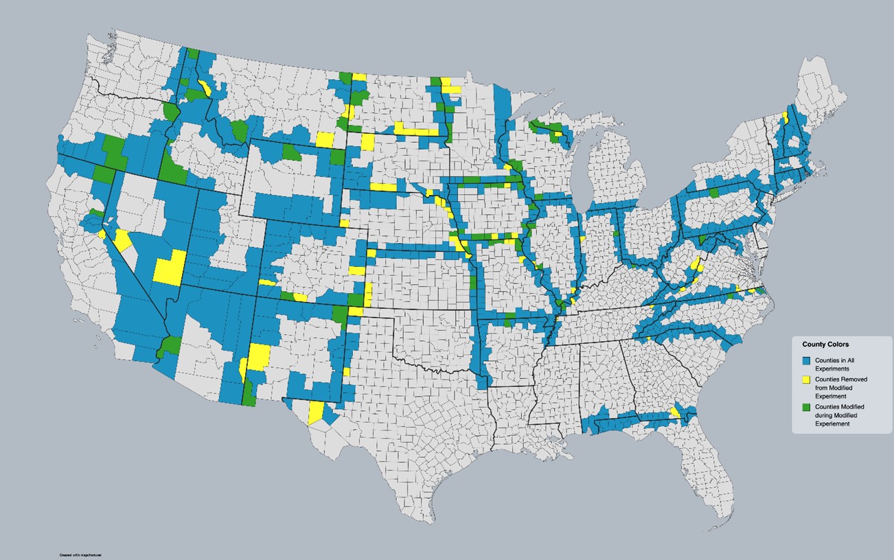
Figure 4: Status of counties in revised experiment. Unchanged Counties are blue, removed counties are yellow, and counties with some removed experiments are green.
Two more variables were added to the revised data set as proxies for labor demand, the state’s median county size and the county’s population (TOTALPOPi,t). The median county size ended up being perfectly multicollinear with county fixed effects and thus was not included in the models. The population data came from the Census Bureau’s Population Estimates. The Census Bureau adopted a different data collection system in 2000 so the data was limited to years after 2000 to accommodate the new variable. Only around two percent of the data was removed, the instances from the 1990s. No county stood out as the best choice for a reference group, so the first one, Baldwin County Alabama, was chosen. For year fixed effects, the year 2000 is the reference group. Model (3) was run on the revised data set without county and year fixed effects. Then, Model (4) was run using the same data as Model (3) but with county and year fixed effects added. Model (5) is the same as Model (4) with a county population variable added. Finally, to explore a percent interpretation model, Model (6) was run with ln(EMPLOYi,t) as the dependent variable. All model results are displayed in Table 3. To conserve space, Table 3 does not give the coefficients for all the county and year fixed effects.
Table 3: Difference in Difference Regression Results for all Minimum Wage Experiments
| Baseline Model (1) |
Baseline Model with Added Fixed Effects (2) |
Revised Data and no Fixed Effects (3) |
Revised Data with Fixed Effects (4) |
Revised Data with Fixed Effects and Pop. Added (5) |
Log-Linear with Revised Data, Fixed Effects, and Pop. Added (6) |
|
|---|---|---|---|---|---|---|
| Variables | EMP | EMP | EMP | EMP | EMP | ln(EMPt) |
| TREATEDi,t | 249.6***
(74.29) |
-28.11
(32.40) |
249.6***
(83.99) |
-8.170 (28.79) | 20.53
(16.94) |
0.00981*
(0.00578) |
| POSTi,t | 32.05
(67.40) |
-2.968 (13.40) | 29.10
(76.23) |
-4.067
(13.71) |
-4.512
(8.761) |
-0.000581 (0.00374) |
| (TREATEDi,t)(POSTi,t ) | -16.49 (106.6) | -2.010 (19.98) | 30.05
(119.8) |
-6.567
(19.32) |
0.0344
(13.74) |
0.00334 (0.00543) |
| TOTALPOPi,t | — | — | — | — | 0.0195*** (0.00108) | 1.08e-06*** (9.79e-08) |
| Constant | 1425*** (75.21) | 1525*** (313.0) | 1595*** (84.72) | -1172*** (340.3) | -1172*** (206.3) | 7.555*** (0.0310) |
| Observations | 14883 | 14883 | 13085 | 13085 | 13083 | 11290 |
| R2 | 0.0043 | 0.968 | 0.005 | 0.976 | 0.988 | 0.991 |
| Adj. R2 | 0.00406 | 0.966 | 0.00443 | 0.974 | 0.987 | 0.990 |
| SER | 3234 | 596.4 | 3414 | 548.8 | 390.8 | 0.143 |
| Fixed Effects | X | X | X | X | ||
| Population Added | X | X | ||||
| Used Revised Data | X | X | X | X |
Revised Data refers to the data pictured in Figure 4 after zeros are removed. The robust standard errors are in parentheses and *** means p<0.01, ** means p<0.05, * means p< 0.1.
VI. MODEL VALIDITY
There are distinct issues with each of these models, but Model (5) tells the most compelling story. Table 4 displays the residuals for Model (5).
Table 4: Summary Statistics for residuals in Model 5
| Mean | Variance | |
|---|---|---|
| $$\hat{u}$$ | 1.06e-7 | 144269.9933 |
| $$\hat{u}$$ when (TREATEDit)(POSTit ) = 1 | 1.25e-7 | 138241.4863 |
| $$\hat{u}$$ when (TREATEDit)(POSTit ) = 0 | 4.96e-8 | 162506.0569 |
The mean for all three rows is essentially zero, meaning the conditional mean independence assumption holds, and the beta coefficients are unbiased. With the removal of uninformative zeros, no instance or set of instances are unduly influencing the regression line, meaning the assumption that large outliers are unlikely is met. No perfect multicollinearity exists in the model because Stata removes any variables that are multicollinear. The year and county fixed effects also have reference groups to avoid multicollinearity. Unfortunately, the data is not independently and identically distributed since it is panel data and thus time dependent. The employment for a county in one year will provide information about the range of potential employment values for that county in the next year. The difference in difference model accounts for the issue by differencing out the time constant error term. Table 4 also indicates that the model suffers from heteroskedasticity. To account for that, heteroskedastic robust errors were used for all the models.
Models (1) and (3) fail the conditional mean independence assumption and thus have biased beta coefficients. When fixed effects are added, the magnitude of these beta coefficients decreases significantly in absolute value, indicating that the coefficients in Models (1) and (3) are overstated. Model (2) is biased because it contains roughly 1800 instances of uninformative zeros. While not technically outliers, having so many zeros that are not relevant unduly influences the regression line. Models (3) and (4) are the same in construction as Models (1) and (2), but they are run on the modified data specified in section 4. Not including total population in Model (4) also introduces omitted variable bias because adding it significantly changed the magnitude and sign of the coefficient of the variable of interest, (TREATEDit)(POSTit ). Thus, Model (4) also fails the conditional mean independence assumption due to omitted variable bias.
The log-linear model (Model (6)) is not the best model because of sample selection bias. To run a logarithmic transformation, all instances where employment was equal to zero must be removed, meaning that data set had missing values based on a value of the dependent variable. These missing values bias the beta coefficients. In Models (3), (4), and (5), uninformative zeros were removed, but removing uninformative zeros is different from removing all of them. The log-linear model is biased, so Model (5) is preferred.
Model (5) also fits the data the best with an adjusted R2 value of 0.987. That is, around 99% of the variability in employment is accounted for by the model. Model (5) also has the lowest SER value of 390.8, meaning this model only mispredicts by 390 people on average. The goodness of fit statistics reveal that the Model 5 tells the most complete story, one that does not provide any evidence that the minimum wage has any impact on employment numbers. In fact, that story indicates that employment is much more reliant on county and year than an increase in the minimum wage.
VII. RESULTS AND CONCLUSIONS
Again, the variable of interest is (TREATEDit)(POSTit ). In every model, the coefficient on the variable of interest is statistically insignificant, meaning the models fail to assert any relationship between the minimum wage and employment. In the models without fixed effects (Models (1) and (3)), TREATEDi,t is the only slope coefficient that is statistically significant. However, these models clearly suffer from omitted variable bias. When compared to the models with county fixed effects (all other models), the coefficient on TREATEDi,t drops significantly, meaning the original coefficient was overstated. The coefficients on (TREATEDit)(POSTit ) decreased in absolute value when fixed effects were added implying the initial beta coefficient estimates for (TREATEDit)(POSTit ) also suffered from omitted variable bias.
In Model (5), the coefficient on (TREATEDit)(POSTit ) becomes the most insignificant of all the models, but also the least biased. As discussed in the model validity section, Model (5) provides the best estimate for the variable of interest. However, even if the coefficient on (TREATEDit)(POSTit ) was statistically significant, it would not be economically significant to say that increasing the minimum wage is associated with an increase of 0.0344 fast food employees.
Regarding the minimum wage debate, recall one side argues that increasing the minimum wage would lead to a decrease in employment. While theoretically true in competitive labor markets, the regression analysis provides no empirical evidence to support that claim using limited-service employment data from 2000-2022. Thus, I suggest tying the minimum wage to inflation. Since a sizable portion of the experiments in this analysis include states that have adopted that policy, I do not expect that policy to reduce employment. Several states already have an effective minimum wage four or five dollars higher than the national minimum so increasing the national minimum wage would not impose a binding price floor on most counties. Also, very few people in the job market earn the minimum wage to begin with. Most minimum wage workers are in food and drink services, which is why the data was restricted to limited-service restaurants in the first place. In the data set, limited-service workers made up approximately one percent of the population of a county on average.
There are some limitations to this work. It’s possible that some counties experience an increase in employment due to minimum wage increases and others experience a decrease. If there are some counties with a substantial increase and others with a substantial decrease, they might be acting against each other, which would result in an insignificant change overall. In the future, robustness tests to evaluate the possibility of different counties’ results negating each other should be conducted. More proxies for labor demand should also be included because elasticity of demand directly impacts theorized reduction in quantity of labor demanded.
While these findings show no statistical significance that moderately increasing the minimum wage will impact employment numbers, future policy changes should also be assessed to verify this paper’s findings. With data being a much larger part of life, researchers with enough foresight will be able to collect data for better proxies of labor demand. For example, if one anticipates an increase in the minimum wage, one could collect data on the number of McDonald’s locations before and after the minimum wage increase. If the next federal minimum wage increase makes the minimum wage $15 an hour, researchers could compare employment numbers in states based on how much the minimum wage changed. For example, if the minimum wage increased to $15 an hour, South Carolina’s effective minimum wage would increase by $7.75 while California’s effective minimum wage would not change. If such a natural experiment were to happen, empirical research on the severity of minimum wage increases and the resulting impact could be pursued, but this study does not provide any insight into the effects of doubling the minimum wage. With the currently available data, no evidence that modest increases in the minimum wage resulted in lower employment was found and therefore I suggest policies to tie minimum wage to inflation.
VIII. REFERENCES
Beaudry, Paul, David A. Green, and Ben M. Sand. “In Search of Labor Demand.” American Economic Review 108, no. 9 (September 1, 2018): 2714–57. https://doi.org/10.1257/aer.20141374.
Brown, Charles. “Minimum Wage Laws: Are They Overrated?” Journal of Economic Perspectives 2, no. 3 (August 1, 1988): 133–45. https://doi.org/10.1257/jep.2.3.133.
Card, David, and Alan B Krueger. “Minimum Wages and Employment: A Case Study of the Fast-Food Industry in New Jersey and Pennsylvania: Reply.” American Economic Review 90, no. 5 (December 1, 2000): 1397–1420. https://doi.org/10.1257/aer.90.5.1397.
Card, David, and Alan Krueger. “Minimum Wages and Employment: A Case Study of the Fast Food Industry in New Jersey and Pennsylvania,” October 1993. https://doi.org/10.3386/w4509.
Dube, Arindrajit, T. William Lester, and Michael Reich. “Minimum Wage Effects Across State Borders: Estimates Using Contiguous Counties.” Review of Economics and Statistics 92, no. 4 (November 2010): 945–64. https://doi.org/10.1162/rest_a_00039.
“Quarterly Census of Employment and Wage 1990-2023.” QCEW. Washington DC, United States: Bureau of Labor Statistics, Accessed September 6, 2023. https://www.bls.gov/cew/downloadable-data-files.htm.
Neumark, David, and William Wascher. “Minimum Wages and Employment: A Case Study of the Fast-Food Industry in New Jersey and Pennsylvania: Comment.” American Economic Review 90, no. 5 (December 1, 2000): 1362–96. https://doi.org/10.1257/aer.90.5.1362.