Volume 33, Issue 1: Paper 3
The Minimum Wage and the Gender Wage Gap in the United States
Roberto Ureña, State University of New York at New Paltz
Since the 1980s, it has been widely assumed that increases in the minimum wage will increase women’s earnings relative to men’s earnings. The reasoning behind this theory is relatively straightforward: Women are more likely to have minimum wage jobs than men, and therefore are more likely to benefit from increases in the minimum wage. There is some evidence that such gender segregation is still the case—seeing as 59% of minimum wage workers are women (Economic Policy Institute 2021). Surprisingly, there has been relatively little research on this topic since the late 1990s. This dearth of research may in part be due to the fact the federal minimum wage has not changed in nominal terms in the United States since 2009. As a result, the theory on the effects of the minimum wage on the gender wage gap has gone largely unchallenged in recent years.
Since that time, however, much has changed. In particular, the United States has experienced an unprecedented number of female college graduates—such that more women are enrolling in and graduating from college than men (Parker 2021). An increase in the number of female graduates, of course, should also mean fewer women working for minimum wage—and thus one would expect fewer women to be directly affected by increases in the minimum wage. While it is true that many women work at minimum wage level jobs, it is less than clear that the number of women who work for minimum wage jobs are sufficient to have a statistically significant impact on women’s earnings in general. There is good reason to be wary: A recent revisiting of the research on this topic has called into question the extent of the effects of the minimum wage on the gender wage gap, finding that the minimum wage has a much smaller effect on the gender wage gap than was previously thought (Autor, Manning, and Smith 2016; hereafter ‘Autor et al’). All of this undermines the longstanding theory that increases in the minimum wage predominately affect women’s earnings.
Of course, the question of the gender wage gap in general is the most discussed topic in feminine economics. A plethora of solutions have been offered as to how to reduce the gender wage gap, most notably by Blau and Kahn (2017). Having considered all of these, however, all have been forced to acknowledge that a sizeable amount of the gender wage gap cannot be explained by any single factor (Blau and Kahn 2017). The number of unobservable characteristics—including sex discrimination—which are difficult to control for in a standard regression, make the task of determining which factors most affect the gender wage gap.
While the gender wage gap in general receives a considerable bit of attention, the question of the effect of the minimum wage in particular on the gender wage gap has gone overlooked. Thus, the hope of this paper—at least in part—is to fill a void in the literature, and to reopen a case which, since the late 1990s, has largely gone cold, particularly in the United States.
II. Literature Review
An explanation for the need for further research in this area necessitates a brief history of the research in this field, seeing as much of the research on this topic—and, in fact, nearly all of the theory—is more than twenty years old.
Card and Krueger (1994) pioneered investigation into the effects of the minimum wage on labor markets, and their work laid the foundations for nearly all research on the minimum wage that followed. In finding that increasing the minimum wage does not, all things being equal, diminish employment rates, Card and Krueger (1994) challenged the traditional assumptions of minimum wage theory and provided the impetus for other researchers to delve into the field. Although the findings of Card and Krueger (1994) are not directly relevant to the topic of this paper, their work in this field must be duly acknowledged—as it has been acknowledged by the scholars whose work this paper more directly builds upon. Published almost simultaneously alongside Card and Krueger (1994), Oaxaca and Ransom (1994), building on the earlier work of Oaxaca (1973), provide the groundwork for the methodology of understanding the effects of discrimination on the race and gender wage gaps. Oaxaca and Ransom (1994) warn against assuming a uniform wage structure when analyzing the effects of wage discrimination at the firm level. Again, while the discriminatory components of the gender wage gap are not the subject of this paper, the methodological foundation provided by Oaxaca and Ransom (1994) forms the basis for many of the researchers who have explored this topic.
The first paper to directly discuss the effects of the minimum wage on the gender wage gap—among other wage gaps—is the seminal article by DiNardo, Fortin, and Lemieux (1996; hereafter DiNardo et al). Three foundational findings emerge from DiNardo et al (1996). First, diminishing real minimum wages from 1979-1988 could explain a “substantial portion of wage inequality, particularly for women” (1001). Second, DiNardo et al (1996) point out that the effects of changes in the real minimum wage are not equally distributed among states: A rising minimum wage has a more substantial impact in low-wage states as supposed to high-wage states (1039). Third, DiNardo et al (1996) note that as education increases, the effects of changes in the minimum wage decrease considerably (1034-35), as one might expect intuitively. Having pointed out the nuances involved in analyzing the effects of the minimum wage, DiNardo et al (1996) conclude that wage inequality is best explained by changes in the minimum wage and unionization rates—all other institutional labor market factors, such as supply and demand, play a “secondary role to such factors as the extent of unionization and the minimum wage” (1040). These findings, alongside the findings of Card and Krueger (1994), reinforce the idea that the traditional supply-and-demand model may not provide the best explanation for the workings of the labor market.
Building directly on the work of DiNardo et al (1996), Lee (1999) uses cross-sectional data to determine whether changes in the minimum wage drives changes in wage inequality among low-wage workers, or whether other factors are involved. The results of Lee’s (1999) research corroborate the findings of DiNardo et al (1996). However, Lee’s (1999) findings raise questions of their own: “The falling relative level of the minimum wage can explain from 70 to 100 percent of the growth in inequality in the lower tail of the female wage distribution” (1016). In other words, changes in the minimum wage could account for all or almost all changes in the low-wage gender wage gap—at least, for women with low levels of human capital.
In contrast to the prior literature, Shannon (1996) argues that the alleged benefit of the minimum wage on reducing wage discrimination might partly be the result of diminished overall employment, particularly among women (1576). Shannon (1996) argues that the minimum wage seems to raise the wages of low-wage adult men, while having negligible or inconclusive effects on the wages of other demographic groups (1575). This suggests that, as predicted by the traditional theory on the minimum wage, that rising wages might be counteracted by falling employment rates.
These findings and their interpretation, of course, conflict with Card and Krueger’s (1994) earlier work, as well as with the work of DiNardo et al’s (1996). Shannon’s (1996) interpretation is, perhaps, a reflection of a more traditional theory of labor economics. Nonetheless, it is not an interpretation which can be readily dismissed. It is interesting to see, however, that in the literature which followed Shannon (1996) is seldom mentioned. Shannon’s (1996) significance, however, lies not in its being foundational to the work which followed, but in providing the first indications of the questionability of the theory espoused by DiNardo et al (1996) and Lee (1999).
After DiNardo (1996), Shannon (1996), and Lee (1999), however, research on the effects of the minimum wage on the gender wage gap ceased. Despite the unanswered questions and disagreements regarding the theory, little new work was done. The literature simply and abruptly fell silent. Some research was done on the effect of a rise in the minimum wage in the United Kingdom in 1975 (Sutherland, Dex, and Joshi 2000; Robinson 2005), but apart from this, little new was said.
More than fifteen years after Lee (1999), Li and Ma (2015) presented their findings on the effects of the minimum wage on the gender wage gap in China, using the methodology put forward by Oaxaca and Ransom (1994). Challenging the findings of the preceding literature, Li and Ma (2015) find that “gender wage gaps in the low-wage distribution groups are greater than are those in middle- and high-wage distribution groups” following an increase in the minimum wage (10). Such findings suggest that the minimum wage, in fact, may actually accentuate the gender wage gap for low-wage workers—at least in the short run. Li and Ma (2015) indicate that this may simply be the result of de facto discrimination against low-wage female workers relative to men (18). If this were the case, then this would corroborate the findings of Shannon (1996). While the discrepancy between these findings and the rest of the literature may be the result of differences in political institutions, Li and Ma’s (2015) results cannot be ignored.
A year later, the traditional literature was again called into question by Autor et al (2016), who—after almost two decades—reviewed the methodology and results of Lee (1999) and find that Lee’s (1999) methodology resulted in severely biased estimates. Using Lee’s (1999) 1979-1988 data set, Autor et al (2016) compare OLS without state fixed effects to a 2SLS approach1, and find that the effects of the minimum wage on the gender wage gap—though still substantial—were not nearly as extreme as those presented by Lee (1999). Compared to Lee’s (1999) estimate that changes in the minimum wage could explain 70-100% of the changes in the low-wage gender wage gap, Autor et al (2016) find that the minimum wage only explain about 30-40% (Autor et al 2016, 61)—still economically significant, but not nearly as extreme as the findings of Lee (1999).
Autor et al (2016) also present other challenges to the approach of Lee (1999), suggesting that the time span of Lee’s (1999) data set was not sufficiently large to adequately measure the effects of the minimum wage (61). Furthermore, Autor et al (2016) hypothesize that—even of the 30-40% effect remaining after Lee’s (1999) methodology was corrected—a significant amount of that effect may have been the result of measurement error (89).
Autor et al (2016) warn that their conclusions, however, were based “on some strong assumptions and so should not be regarded as definitive” (88). Nevertheless, Autor et al’s (2016) work, coupled with the earlier and independent work of Shannon (1996), casts serious doubt on the findings of Lee (1999), as well as the findings of the prior literature.
The findings of the most recent literature have not brought much closure to these issues. Few new studies have estimated the gender wage gap for workers, and so much of the research has been done internationally. In Poland, Majchrowska and Strawiński (2018) find that the minimum wage hike lowers the gender wage gap among younger workers, with little to no effect for more experienced, higher skilled workers (183), lending support to the older theory put forward by DiNardo et al (1996).
In Japan, Kawaguchi and Mori (2021)—while not directly considering the effects of the minimum wage on the gender wage gap—find that Japan’s minimum wage2 has a positive impact on the wages of young workers, though this effect is somewhat counterbalanced by a negative impact on the employment of less-educated men (388). These results bolster the conclusions of Shannon (1996) and challenge the DiNardo et al (1996) findings, and again provide some evidence that the effects of the minimum wage on wage inequality may not be as substantial as the data suggests.
In Germany, Caliendo and Wittbrodt (2021), in attempting to replicate the work of Li and Ma (2015) and Majchrowska and Strawiński (2018), find that increases in the minimum wage in fact do diminish the gender wage gap at higher levels of income, education, and skill, even if the effects are somewhat smaller. These results, while somewhat contrary to the findings of Majchrowska and Strawiński (2018), do not otherwise defect from the preexisting literature.
What can be seen, then, is a strange narrative with numerous holes and myriad questions left to be answered. The paucity of empirical studies and the conflicting evidence in those studies have been bemoaned by the scholars in the field (Autor et al 2016, 59). Research on the effects of the minimum wage on the gender wage gap—particularly for the U.S.—is desperately needed. This paper seeks to meet that need. Of course, while no single paper can provide conclusive results on this topic—especially as the findings in the field have been so varied—this paper hopes to provide evidence as to whether the traditional theory on this issue is correct, or whether it needs to be revised.
III. Data and Methodology
A. Sample Data
This paper will use the Current Population Survey (CPS), retrieved from the IPUMS database. The CPS is the primary source of data on labor statistics in the United States (Harvard University 2022), and is commonly used by scholars studying the gender wage gap—including Lee (1999) and Autor, Manning, and Smith (2016), whose research represents part of the basis for the present study. The CPS conducts monthly surveys at the household level, collecting data on each individual in the household. The January 2023 micro-data which will be used for this analysis includes 99,337 individuals in 68,726 households. This paper will use cross-sectional micro-level data to report changes in earnings at the individual level.
Although Blau and Kahn (2017) point out that a large part of the gender wage gap can be explained by differences in pay between part-time and full-time workers, this paper will not drop part-time workers from the sample. This is because the general theory on the effect of the minimum wage on the gender wage gap indicates that the primary effect of the minimum wage is on young workers—and one would expect young workers to be disproportionately part-time workers (Hansen 2005). Thus, this paper will instead include in the work force, and control for full-time status using a full-time worker dummy variable.
Table 1 contains the descriptive statistics for this sample.3 The average age of workers in the sample is about 43 years old, with a minimum age of 16 and a maximum age of 85. Since all individuals outside of the work force have been dropped, a maximum age of 85 for this sample, even though most individuals retire at around the age of 65. Notice that approximately 48% of the sample is female, as supposed to 50.5% of the total U.S. population (U.S. Census Bureau). This 2 to 3% difference will, in all likelihood, prove to be insignificant, but when considering whether or not the sample is representative of the population, should be kept in mind.
Table 1: Descriptive Statistics for Sample
| Variable | Obs | Mean | Std. Dev. | Min | Max |
|---|---|---|---|---|---|
| Weekly Earnings | 10187 | 1178.977 | 762.989 | .01 | 2884.61 |
| Age | 10187 | 42.505 | 14.618 | 16 | 85 |
| Female | 10187 | .49 | .5 | 0 | 1 |
| Union Worker | 10187 | .101 | .302 | 0 | 1 |
| Associate’s Degree | 10187 | .256 | .437 | 0 | 1 |
| Bachelor’s Degree | 10187 | .257 | .437 | 0 | 1 |
| Master’s Degree | 10187 | .113 | .317 | 0 | 1 |
| Professional Degree | 10187 | .017 | .129 | 0 | 1 |
| Doctorate Degree | 10187 | .027 | .162 | 0 | 1 |
| White | 10187 | .795 | .403 | 0 | 1 |
| Marital Status | 10187 | .517 | .5 | 0 | 1 |
| Full-time Worker | 10187 | .779 | .415 | 0 | 1 |
| Urban Status | 10187 | .663 | .473 | 0 | 1 |
| Blue State | 10187 | .462 | .499 | 0 | 1 |
| Red State | 10187 | .431 | .495 | 0 | 1 |
| Purple State | 10187 | .107 | .31 | 0 | 1 |
Furthermore, notice that unionization rates in this sample are at approximately 2%, as compared with about 9-11% of the overall population (U.S. Bureau of Labor Statistics: “Economic News Release”). This was largely due to data-related factors—there were a large number of missing values for the unionization rate variable on CPS for the January 2023 micro-data. This discrepancy is very significant. Considering that DiNardo et al (1976) suggest that unionization is one of the primary factors involved in determining the effect of the minimum wage on the gender wage gap (1040), this paper will ultimately regress union rates on earnings. However, this error in the data must be remembered when considering the results of this study.
Tables 2 and 3 summarize the sample statistics by sex. Notice that about 60% of both males and females live in states with minimum wages higher than the federal minimum wage (indicated by the ‘Minimum Wage’ line). Further comparison between the two sample statistics reveals a rather interesting picture. First, there is a quite visible gender wage gap, with males earning on average about $1314.76 per week, and females earning on average about $1037.68. Despite the size of the standard deviations, this discrepancy is nonetheless striking. Second, notice that females appear to be better educated than males on average. Males are more likely to hold as their highest educational attainment a high-school diploma or lower. Females have more of every other kind of degree except for professional degrees—for which they are equal with males—and doctorate degrees. Third, notice that men are more likely than women to work full-time—which is a well-documented phenomenon in the literature on the gender wage gap (Blau and Kahn 2017, Chung 2018), as has already been pointed out.
Table 2: Descriptive Statistics: Male
| Variable | Obs | Mean | Std. Dev. | Min | Max |
|---|---|---|---|---|---|
| Weekly Earnings | 5195 | 1314.757 | 789.363 | .01 | 2884.61 |
| Age | 5195 | 42.183 | 14.591 | 16 | 85 |
| Female | 5195 | 0 | 0 | 0 | 0 |
| Union Worker | 5195 | .104 | .305 | 0 | 1 |
| Associate’s Degree | 5195 | .243 | .429 | 0 | 1 |
| Bachelor’s Degree | 5195 | .244 | .43 | 0 | 1 |
| Master’s Degree | 5195 | .094 | .292 | 0 | 1 |
| Professional Degree | 5195 | .018 | .133 | 0 | 1 |
| Doctorate Degree | 5195 | .029 | .169 | 0 | 1 |
| White | 5195 | .816 | .388 | 0 | 1 |
| Marital Status | 5195 | .534 | .499 | 0 | 1 |
| Full-time Worker | 5195 | .831 | .375 | 0 | 1 |
| Urban Status | 5195 | .664 | .473 | 0 | 1 |
| Blue State | 5195 | .462 | .499 | 0 | 1 |
| Red State | 5195 | .43 | .495 | 0 | 1 |
| Purple State | 5195 | .107 | .309 | 0 | 1 |
Table 3: Descriptive Statistics: Female
| Variable | Obs | Mean | Std. Dev. | Min | Max |
|---|---|---|---|---|---|
| Weekly Earnings | 4992 | 1037.676 | 707.462 | 1 | 2884.61 |
| Age | 4992 | 42.839 | 14.639 | 16 | 85 |
| Female | 4992 | 1 | 0 | 1 | 1 |
| Union Worker | 4992 | .099 | .298 | 0 | 1 |
| Associate’s Degree | 4992 | .27 | .444 | 0 | 1 |
| Bachelor’s Degree | 4992 | .271 | .444 | 0 | 1 |
| Master’s Degree | 4992 | .133 | .339 | 0 | 1 |
| Professional Degree | 4992 | .016 | .125 | 0 | 1 |
| Doctorate Degree | 4992 | .024 | .153 | 0 | 1 |
| White | 4992 | .774 | .418 | 0 | 1 |
| Marital Status | 4992 | .499 | .5 | 0 | 1 |
| Full-time Worker | 4992 | .725 | .447 | 0 | 1 |
| Urban Status | 4992 | .662 | .473 | 0 | 1 |
| Blue State | 4992 | .461 | .499 | 0 | 1 |
| Red State | 4992 | .431 | .495 | 0 | 1 |
| Purple State | 4992 | .108 | .31 | 0 | 1 |
To measure minimum wages at the state level, this paper uses data provided by the U.S. Department of Labor. Table 4 summarizes the state data. Notice that the lowest level of minimum wage is $7.25, which is the federal minimum wage. There are 20 states with minimum wages at the federal level. It should be noted, however, that differences in state minimum wages are highly correlated with the political orientation of that state (Ford, Minor, and Owens 2012). This, of course, raises the problem of the endogeneity of the minimum wage. To address this concern, the political orientation of the state and the GDP of that state will be evaluated as potential factors which may affect the minimum wage of a particular state. Given that neither of these factors are theoretically significant to the discussion of the effects of the minimum wage on the gender wage gap, the concern here will be with the statistical significance of these variables. Those variables which are found to be statistically significant will be included in the final regression.
Table 5 shows a regression of the political orientation of states on minimum wages. There are three types of political orientation: ‘Red States,’ ‘Blue States,’ and ‘Purple States.’ A ‘Red State’ is defined as a state for which both U.S. Senators of that state identify as Republicans, a ‘Blue State’ is defined as a state for which both U.S. Senators of that state identify as Democratic, and a ‘Purple State’ is defined as a state for which one U.S. Senator of that state identifies as Republican, and the other identifies as Democratic.4 Although this is a somewhat arbitrary definition, it is sufficient for the present purpose of providing a clean distinction between states along political lines. It should be noted that, for the regressions, purple states will not be included, as including red, blue, and purple state dummy variables would result in redundancy—on the definitions here established, all states are either red, blue, or purple. Thus, the coefficients of red and blue states are in comparison to purple states in the regressions which include the political orientation variable. It is interesting to note that, on the definition established, and as might have been expected, blue states average substantially higher minimum wages than red states—with purple states between the two. This correlation is statistically significant and does in fact seem to be economically significant as well. Thus, it is necessary to control for the political orientation of the state in this study’s final regression.
Table 4: Descriptive Statistics for Minimum Wage
| Variable | Obs | Mean | Std. Dev. | Min | Max |
| Minimum Wage | 51 | 10.415 | 2.973 | 7.25 | 16.5 |
|---|
Table 5: Minimum Wage by Political Orientation of State
| Minimum Wage | Coef. | St.Err. | t-value | p-value | [95% Conf | Interval] | Sig |
| Red State | -1.237 | .98 | -1.26 | .213 | -3.208 | .734 | |
|---|---|---|---|---|---|---|---|
| Blue State | 3.176 | .976 | 3.26 | .002 | 1.215 | 5.138 | *** |
| Constant | 9.517 | .869 | 10.95 | 0 | 7.77 | 11.264 | *** |
| Mean dependent var | 10.415 |
|---|---|
| R-squared | 0.508 |
| F-test | 24.782 |
| Akaike crit. (AIC) | 224.685 |
| SD dependent var | 2.973 |
| Number of obs | 51 |
| Prob > F | 0.000 |
| Bayesian crit. (BIC) | 230.481 |
*** p<.01, ** p<.05, * p<.1
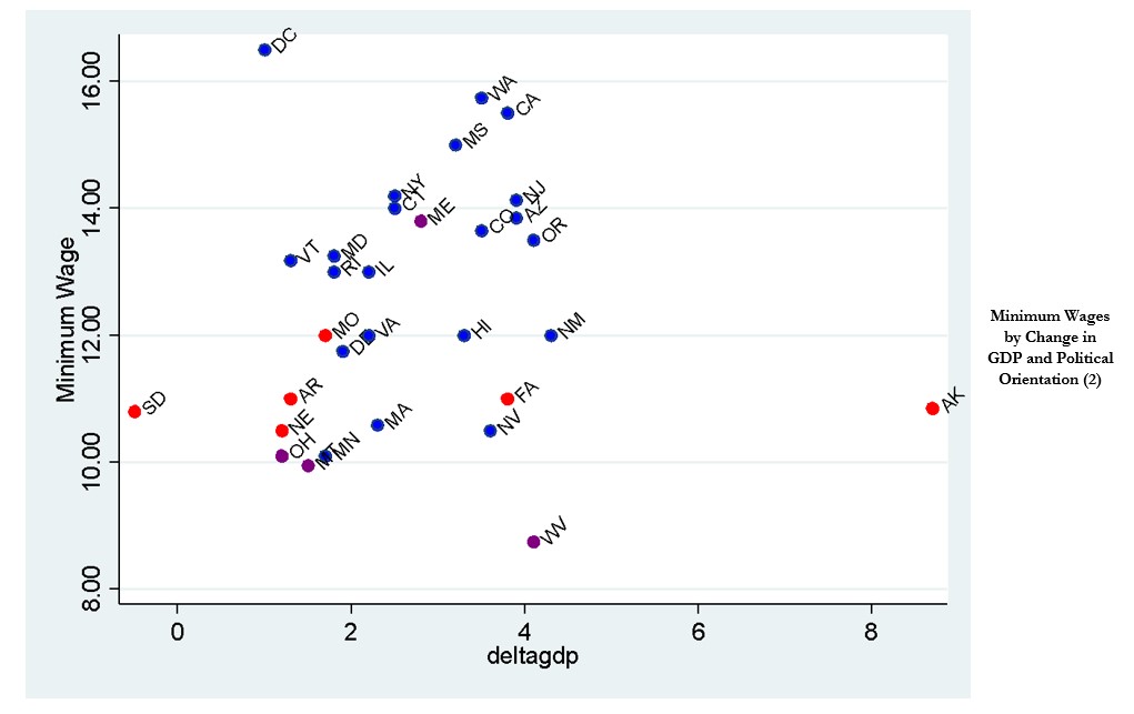
The correlation of political orientation and minimum wages in states may, however—as previously mentioned—have to do with other endogenous factors within states, such as state GDP, which may also serve as a proxy for cost-of-living in general. Table 6 describes the regression of state GDP—defined as the percent change in GDP over a particular economic quarter—on minimum wages. Figure 2 in the Appendix charts this correlation, color-coding each state by its political orientation. For this graph, those states at the federal minimum wage level have been excluded. Although one can see that, on average, as the percent change in GDP increases, the minimum wage also increases, the correlation is not statistically significant. As such, for this paper, the final regression will not control for the GDP of the state.
Table 6: Minimum Wage and Percent Change in GDP
| Minimum Wage | Coef. | St.Err. | t-value | p-value | [95% Conf | Interval] | Sig |
|---|---|---|---|---|---|---|---|
| % Change in GDP | .069 | .222 | 0.31 | .757 | -.384 | .523 | |
| Constant | 12.27 | .697 | 17.60 | 0 | 10.844 | 13.696 | *** |
| Mean dependent var | 12.458 |
|---|---|
| R-squared | 0.003 |
| F-test | 0.097 |
| Akaike crit. (AIC) | 131.761 |
| SD dependent var | 1.934 |
| Number of obs | 31 |
| Prob > F | 0.757 |
| Bayesian crit. (BIC) | 134.629 |
*** p<.01, ** p<.05, * p<.1
B. Methodology
Methodologically, this paper will use OLS. Autor et al (2016) warns against using OLS without state fixed effects—chiefly as a critique of Lee (1999) (Autor et al 2016, 71). While Autor et al (2016) recommended 2SLS, this paper will use OLS, but will—unlike Lee (1999)—include state fixed effects. This is because the main potential choice variable which will be used in the regression is the political orientation of the state in which the individual resides—which, as aforementioned, is correlated with the minimum wage of the state—raising the potential for endogeneity bias. However, it is well known that when instrumental variables are weak, the bias generated by 2SLS is often greater than the coefficient bias generated by OLS (Angrist and Krueger 2001; Hahn and Hausman 2003). As far as the author is aware, there are no strong or commonly used instrumental variables for the state minimum wage. As such, this paper will regress using OLS rather than 2SLS.
C. Regressing Equation
The methodology of this paper will be based on the Mincerian wage equation (Mincer 1974), which relates wages to experience and education. This Mincerian wage equation has become a commonly used foundation for wage equations (Borjas 2013, 276-277). Mincer’s wage equation shows that wages are related to experience and education in the form:
(1) $$ln\ w\ =\ \beta_1s\ +\ \beta_2t\ – β3t2 + Other Variables$$
where w is the worker’s wage rate, s is the number of years in school, and t is time spent in the workforce. The variable t is represented both linearly and exponentially in order to capture the diminishing marginal product of time spent in the workforce on productivity—increasing rapidly in the early years, as workers quickly learn and increase in productivity, and then eventually flattening out as time in the workforce increases (Borjas 2013, 277). Also, for the purposes of this paper, s will be subdivided into five dummy variables—one for Associate’s Degree, Bachelor’s Degree, Master’s Degree, Professional Degree, and Doctorate Degree—taking a value of 1 if the individual has attained the level of education specified, and taking a value of 0 for all educational levels less than a completed Associate’s Degree. Furthermore, because the CPS does not include data for time in the workforce, in this paper, ‘age’ will be used as a proxy for time spent in the workforce. Age is a well-known and commonly used proxy for time in the workforce in wage theory, despite the measurement error involved (Zveglich, et al. 2019). The assumption of this paper is that most individuals will begin working as soon as they are legally able to—that is, at the age of 16—which is the minimum age of the sample anyway. While this is clearly not the case, the measurement error involved will not affect the estimates themselves, but will only increase the standard errors. Seeing as ‘age’ remains statistically significant at the 1% level in all of the regressions, however, ‘age’ will be considered a sufficient proxy for the present purposes.
Building upon the standard Mincerian wage equation, this paper will estimate using the following wage equation:
(2) $$ln\ w=\ \beta_1s+\ \beta_2t-\beta_3t^2+\ \beta_4Female+\ \beta_5Race+\ \beta_6INT_1+\ \beta_7\aleph$$
where Female is a dummy variable taking a value of 1 if the individual is a female, Race is a dummy variable taking a value of 1 if the individual identifies as white, and where β6INT1 is an interactive variable between the female dummy variable and a minimum wage dummy variable which takes the value of 1 if the state in which the individual lives has a minimum wage higher than the federal level. Furthermore, β7ℵ is a conglomeration of variables, those being: 1) a dummy variable for full-time workers, 2) a variable controlling for the industry in which the individual works, 3) a dummy variable taking a value of 1 if the individual lives in a metropolitan area, and 4) dummy variables for the political orientation of the state of the individual—with ‘political orientation’ defined as previously defined.
Notice, however, that this regression considers the effects of the minimum wage on the gender wage gap, but does not consider the degree to which different increases in the minimum wage may affect the gender wage gap. That is to say, a $1 increase in the minimum wage from $10 to $11 may differ in its impact from a $1 increase from $11 to $12. To estimate the average value of an increase in the minimum wage, this paper will separately regress the following Mincerian wage equation:
(3) $$ln\ w=\ \beta_1s+\ \beta_2t-\beta_3t^2+\ \beta_4Female+\ \beta_5Race+\ \beta_6INT_2+\ \beta_7\aleph$$
where β6INT2 is an interactive variable between the female dummy variable and the natural log of the minimum wage of a given state minus the federal minimum wage.5 Because a log of 0 is not possible, those states at the federal minimum wage level have received values of 0.000001.6
D. Interpreting Dummy Variable Coefficients
Because the dependent variable is a natural log function, the coefficients on all dummy variables will be interpreted based on the following logarithmic approximation:
(4) $$100\ \ 🞄 (exp(β)⬚-1)$$
where exp(β) indicates the mathematical function ‘e,’ raised to the power of the coefficient.
IV. Results
Table 7 details the results of the regression expressed in Equation (2). In particular, notice the ‘Interactive Variable 1’ variable, the ‘Female’ variable, and the ‘Union Worker’ variable. Note that in this equation, after interpreting the coefficients based on the logarithmic approximation stated above, union workers earn about 8.8% more than non-union workers—even after controlling for industry—which is lower than the findings of other studies (e.g., Blanchflower and Bryson 2004; U.S. Department of Labor), and may have to do with the discrepancy in the CPS union data. For this first equation, the gender wage gap is about 18.3%, which seems extraordinarily high—and is, as one might expect, statistically significant—such that an individual who is female, ceteris paribus, earns 18.3% less than her male counterparts. In addition to this, the coefficient on ‘Interactive Variable 1’ is a positive 2.2—even after the logarithmic approximation—which would indicate that if a state has a minimum wage above the federal minimum wage, the gender wage gap decreases by about 2.2%. It must be noted, however, that this ‘Interactive Variable 1’ is not statistically significant. Thus, we cannot reject the null hypothesis that the effects of having a minimum wage greater than the federal minimum wage on the gender wage gap are greater than or equal to 0.
Table 7: Effects of Minimum Wage on the Gender Wage Gap
| lnearnweek | Coef. | St.Err. | t-value | p-value | [95% Conf | Interval] | Sig |
|---|---|---|---|---|---|---|---|
| Female*Minimum Wage | .022 | .024 | 0.92 | .359 | -.025 | .07 | |
| Female | -.169 | .019 | -8.79 | 0 | -.206 | -.131 | *** |
| Minimum Wage | .05 | .063 | 0.79 | .427 | -.074 | .174 | |
| Union | .084 | .018 | 4.68 | 0 | .049 | .12 | *** |
| Age | .053 | .003 | 17.62 | 0 | .047 | .059 | *** |
| Age Squared | -.001 | 0 | -16.46 | 0 | -.001 | 0 | *** |
| Associate’s Degree | .1 | .017 | 5.96 | 0 | .067 | .133 | *** |
| Bachelor’s Degree | .384 | .018 | 20.82 | 0 | .348 | .421 | *** |
| Master’s Degree | .53 | .023 | 22.96 | 0 | .485 | .576 | *** |
| Professional Degree | .597 | .054 | 11.10 | 0 | .491 | .702 | *** |
| Doctorate Degree | .735 | .033 | 22.60 | 0 | .671 | .799 | *** |
| White | .08 | .015 | 5.14 | 0 | .049 | .11 | *** |
| Marital Status | .059 | .013 | 4.50 | 0 | .033 | .085 | *** |
| Full-time Worker | .674 | .02 | 33.93 | 0 | .635 | .713 | *** |
| Urban Status | .046 | .016 | 2.88 | .004 | .015 | .078 | *** |
| Blue State | -.034 | .099 | -0.35 | .728 | -.228 | .159 | |
| Red State | -.12 | .052 | -2.31 | .021 | -.221 | -.018 | ** |
| Constant | 4.711 | .177 | 26.59 | 0 | 4.363 | 5.058 | *** |
| Mean dependent var | 6.824 |
|---|---|
| R-squared | 0.482 |
| F-test | . |
| Akaike crit. (AIC) | 18482.314 |
| SD dependent var | 0.808 |
| Number of obs | 10187 |
| Prob > F | . |
| Bayesian crit. (BIC) | 20716.034 |
*** p<.01, ** p<.05, * p<.1This says nothing, however, about the effects of an increase in the minimum wage on the gender wage gap overall. The previous regression assumes a uniform effect for all minimum wages over the federal level. There is no reason, however, for making this assumption. Table 8 , thus, regresses the effects of different levels of the minimum wage on the gender wage gap using Equation (3). Given the alteration in the interactive variable, it is interesting to note that the gender wage gap, by this framework, has been reduced to approximately 15.8% after the logarithmic approximation has been applied. Furthermore, the impact of the minimum wage has, in fact, decreased as well, to about a fifth of a percent—and, once again, it is not statistically significant. Curiously, the coefficient on the minimum wage premium is -0.8%, and is significant at the 5% level. In any case, we may thus, once more, reject the null hypothesis that the effect of increases of the minimum wage on the gender wage is greater-than or equal to 0.
Table 8: Effects of Minimum Wage Premium on the Gender Wage Gap
| lnearnweek | Coef. | St.Err. | t-value | p-value | [95% Conf | Interval] | Sig |
|---|---|---|---|---|---|---|---|
| Female*Minimum Wage Premium | .002 | .002 | 1.12 | .265 | -.001 | .005 | |
| Female | -.147 | .015 | -9.67 | 0 | -.177 | -.117 | *** |
| Minimum Wage Premium | -.008 | .004 | -2.03 | .042 | -.016 | 0 | ** |
| Union Worker | .084 | .018 | 4.68 | 0 | .049 | .119 | *** |
| Age | .053 | .003 | 17.62 | 0 | .047 | .059 | *** |
| Age Squared | -.001 | 0 | -16.46 | 0 | -.001 | 0 | *** |
| Associate’s Degree | .1 | .017 | 5.96 | 0 | .067 | .133 | *** |
| Bachelor’s Degree | .384 | .018 | 20.82 | 0 | .348 | .421 | *** |
| Master’s Degree | .53 | .023 | 22.97 | 0 | .485 | .576 | *** |
| Professional Degree | .597 | .054 | 11.10 | 0 | .491 | .702 | *** |
| Doctorate Degree | .735 | .033 | 22.61 | 0 | .672 | .799 | *** |
| White | .08 | .015 | 5.15 | 0 | .049 | .11 | *** |
| Marital Status | .059 | .013 | 4.49 | 0 | .033 | .085 | *** |
| Full-time Worker | .674 | .02 | 33.94 | 0 | .635 | .713 | *** |
| Urban Status | .046 | .016 | 2.87 | .004 | .015 | .078 | *** |
| Blue State | .145 | .078 | 1.85 | .064 | -.008 | .298 | * |
| Red State | -.119 | .052 | -2.31 | .021 | -.221 | -.018 | ** |
| Constant | 4.598 | .179 | 25.73 | 0 | 4.248 | 4.948 | *** |
| Mean dependent var | 6.824 |
| R-squared | 0.482 |
| F-test | . |
| Akaike crit. (AIC) | 18481.88 |
| SD dependent var | 0.808 |
| Number of obs | 10187 |
| Prob > F | . |
| Bayesian crit. (BIC) | 20715.608 |
*** p<.01, ** p<.05, * p<.1
It is notable that only the Red State coefficient is significant at the 5% level in both equations, and not the Blue State coefficient. Table 9 regresses the effects of the minimum wage on the gender wage gap using Equation (3), with one exception: Instead of using , Table 9 regresses using , which is an interactive variable between the minimum wage premium, the female dummy, and the red state dummy, and does not contain the blue state variable. This new interaction produces no novel results: The gender wage gap remains at about 16.8% after the logarithmic approximation is applied, and the effect of the minimum wage is both small and insignificant. Furthermore, while the ‘Red State’ coefficient remains significant, and the gender wage gap remains about the same, the interactive variable has a coefficient of exactly 0. Table 10 regresses Equation (3), with the exception that has been replaced with : an interactive variable between the minimum wage premium, the female dummy, and the blue state dummy. This regression does not contain the red state variable. The results are as expected: For the interactive variable, the minimum wage premium, and the blue state variable, the coefficients are small and statistically insignificant. Thus, there is evidence that whether one is in a blue state or a red state, the effect of the minimum wage on the gender wage gap is both statistically and economically insignificant.
Table 9: Effects of Minimum Wage on the Gender Wage Gap in Red States
| lnearnweek | Coef. | St.Err. | t-value | p-value | [95% Conf | Interval] | Sig |
|---|---|---|---|---|---|---|---|
| Female*Minimum Wage Premium*Red States | 0 | .002 | -0.01 | .989 | -.004 | .003 | |
| Female | -.155 | .015 | -10.14 | 0 | -.185 | -.125 | *** |
| Minimum Wage Premium | -.007 | .004 | -1.86 | .063 | -.015 | 0 | * |
| Union Worker | .085 | .018 | 4.70 | 0 | .049 | .12 | *** |
| Age | .053 | .003 | 17.64 | 0 | .047 | .059 | *** |
| Age Squared | -.001 | 0 | -16.47 | 0 | -.001 | 0 | *** |
| Associate’s Degree | .1 | .017 | 5.97 | 0 | .067 | .133 | *** |
| Bachelor’s Degree | .384 | .018 | 20.82 | 0 | .348 | .421 | *** |
| Master’s Degree | .53 | .023 | 22.96 | 0 | .485 | .576 | *** |
| Professional Degree | .597 | .054 | 11.10 | 0 | .492 | .702 | *** |
| Doctorate Degree | .735 | .033 | 22.59 | 0 | .671 | .799 | *** |
| White | .08 | .015 | 5.14 | 0 | .049 | .11 | *** |
| Marital Status | .059 | .013 | 4.50 | 0 | .033 | .085 | *** |
| Full-time Worker | .674 | .02 | 33.93 | 0 | .635 | .713 | *** |
| Urban Status | .046 | .016 | 2.89 | .004 | .015 | .078 | *** |
| Red State | -.121 | .053 | -2.27 | .023 | -.225 | -.016 | ** |
| Constant | 4.602 | .179 | 25.75 | 0 | 4.252 | 4.952 | *** |
| Mean dependent var | 6.824 |
|---|---|
| R-squared | 0.482 |
| F-test | . |
| Akaike crit. (AIC) | 18483.184 |
| SD dependent var | 0.808 |
| Number of obs | 10187 |
| Prob > F | . |
| Bayesian crit. (BIC) | 20716.904 |
*** p<.01, ** p<.05, * p<.1
There is another possibility which may be impacting the results: the regression controls for political orientation, while simultaneously controlling for state fixed effects. It is possible, however, that these state fixed effects are predominately factors determined by or correlated with the political orientation of the state, and are thus resulting in multicollinearity. This may be the reason why the coefficient on the effect of the minimum wage on the gender wage gap is insignificant. While Autor et al (2016) warn against using OLS without state fixed effects, the inclusion of the political orientation variables may serve the same purpose as state fixed effects. Thus, Tables 11 and 12 regress Equation (2) with and, respectively, without state fixed effects. Here we find comparable results to those found previously—the effect of the minimum wage on the gender wage gap remains insignificant.
Table 10: Effects of Minimum Wage on the Gender Wage Gap in Blue States
| lnearnweek | Coef. | St.Err. | t-value | p-value | [95% Conf | Interval] | Sig |
|---|---|---|---|---|---|---|---|
| Female*Minimum Wage Premium*Blue State | .006 | .004 | 1.59 | .113 | -.002 | .014 | |
| FEMALE | -.157 | .013 | -12.07 | 0 | -.182 | -.131 | *** |
| MWP | .001 | .004 | 0.28 | .782 | -.006 | .008 | |
| UNION | .084 | .018 | 4.68 | 0 | .049 | .119 | *** |
| age | .053 | .003 | 17.61 | 0 | .047 | .059 | *** |
| agesquared | -.001 | 0 | -16.45 | 0 | -.001 | 0 | *** |
| ASSO | .101 | .017 | 5.99 | 0 | .068 | .134 | *** |
| BACH | .384 | .018 | 20.83 | 0 | .348 | .421 | *** |
| MAST | .531 | .023 | 22.96 | 0 | .485 | .576 | *** |
| PROF | .597 | .054 | 11.09 | 0 | .491 | .702 | *** |
| DOC | .735 | .032 | 22.63 | 0 | .672 | .799 | *** |
| WHITE | .079 | .015 | 5.12 | 0 | .049 | .11 | *** |
| MAR | .059 | .013 | 4.49 | 0 | .033 | .085 | *** |
| FT | .675 | .02 | 33.95 | 0 | .636 | .713 | *** |
| URB | .046 | .016 | 2.88 | .004 | .015 | .078 | *** |
| BLUE | .123 | .079 | 1.56 | .118 | -.031 | .278 | |
| Constant | 4.6 | .178 | 25.77 | 0 | 4.25 | 4.95 | *** |
| Mean dependent var | 6.824 |
|---|---|
| R-squared | 0.482 |
| F-test | . |
| Akaike crit. (AIC) | 18480.612 |
| SD dependent var | 0.808 |
| Number of obs | 10187 |
| Prob > F | . |
| Bayesian crit. (BIC) | 20714.332 |
*** p<.01, ** p<.05, * p<.1
Table 11: Effects of Minimum Wage on the Gender Wage Gap—No State Fixed Effects
| lnearnweek | Coef. | St.Err. | t-value | p-value | [95% Conf | Interval] | Sig |
|---|---|---|---|---|---|---|---|
| Female*Minimum Wage | .024 | .024 | 1.00 | .316 | -.023 | .072 | |
| Female | -.172 | .019 | -9.03 | 0 | -.21 | -.135 | *** |
| Minimum Wage | .019 | .02 | 0.97 | .331 | -.019 | .057 | |
| Union Worker | .086 | .018 | 4.85 | 0 | .051 | .121 | *** |
| Age | .053 | .003 | 17.45 | 0 | .047 | .058 | *** |
| Age Squared | -.001 | 0 | -16.34 | 0 | -.001 | 0 | *** |
| Associate’s Degree | .1 | .017 | 5.98 | 0 | .067 | .132 | *** |
| Bachelor’s Degree | .386 | .018 | 21.09 | 0 | .35 | .422 | *** |
| Master’s Degree | .538 | .023 | 23.37 | 0 | .493 | .583 | *** |
| Professional Degree | .616 | .054 | 11.48 | 0 | .511 | .722 | *** |
| Doctorate Degree | .746 | .033 | 22.87 | 0 | .682 | .81 | *** |
| White | .076 | .015 | 5.18 | 0 | .047 | .105 | *** |
| Marital Status | .057 | .013 | 4.34 | 0 | .031 | .083 | *** |
| Full-time Worker | .674 | .02 | 33.96 | 0 | .635 | .713 | *** |
| Urban Status | .058 | .014 | 4.23 | 0 | .031 | .085 | *** |
| Blue State | .061 | .02 | 3.01 | .003 | .021 | .101 | *** |
| Red State | .005 | .02 | 0.25 | .804 | -.033 | .043 | |
| Constant | 4.64 | .174 | 26.60 | 0 | 4.298 | 4.982 | *** |
| SD dependent var | 0.808 |
|---|---|
| Number of obs | 10187 |
| Prob > F | . |
| Bayesian crit. (BIC) | 20382.055 |
| Mean dependent var | 6.824 |
| R-squared | 0.477 |
| F-test | . |
| Akaike crit. (AIC) | 18488.092 |
*** p<.01, ** p<.05, * p<.1
Table 12: Effects of Minimum Wage Premium on the Gender Wage Gap—No State Fixed Effects
| lnearnweek | Coef. | St.Err. | t-value | p-value | [95% Conf | Interval] | Sig |
|---|---|---|---|---|---|---|---|
| Female*Minimum Wage Premium | .002 | .002 | 1.19 | .232 | -.001 | .005 | |
| Female | -.149 | .015 | -9.81 | 0 | -.178 | -.119 | *** |
| Minimum Wage Premium | .001 | .001 | 1.00 | .319 | -.001 | .004 | |
| Union Worker | .086 | .018 | 4.83 | 0 | .051 | .121 | *** |
| Age | .052 | .003 | 17.43 | 0 | .047 | .058 | *** |
| Age Squared | -.001 | 0 | -16.32 | 0 | -.001 | 0 | *** |
| Associate’s Degree | .1 | .017 | 5.99 | 0 | .067 | .132 | *** |
| Bachelor’s Degree | .386 | .018 | 21.09 | 0 | .35 | .422 | *** |
| Master’s Degree | .538 | .023 | 23.38 | 0 | .493 | .583 | *** |
| Professional Degree | .616 | .054 | 11.47 | 0 | .511 | .721 | *** |
| Doctorate Degree | .746 | .033 | 22.86 | 0 | .682 | .81 | *** |
| White | .077 | .015 | 5.20 | 0 | .048 | .105 | *** |
| Marital Status | .057 | .013 | 4.36 | 0 | .031 | .083 | *** |
| Full-time Worker | .674 | .02 | 33.97 | 0 | .635 | .713 | *** |
| Urban Status | .057 | .014 | 4.14 | 0 | .03 | .083 | *** |
| Blue State | .059 | .02 | 2.90 | .004 | .019 | .1 | *** |
| Red State | .007 | .02 | 0.33 | .739 | -.032 | .045 | |
| Constant | 4.659 | .175 | 26.60 | 0 | 4.316 | 5.002 | *** |
| SD dependent var | 0.808 |
|---|---|
| Number of obs | 10187 |
| Prob > F | . |
| Bayesian crit. (BIC) | 20381.103 |
| Mean dependent var | 6.824 |
| R-squared | 0.477 |
| F-test | . |
| Akaike crit. (AIC) | 18487.139 |
*** p<.01, ** p<.05, * p<.1
Table 13: Effects of Minimum Wage Premium on the Gender Wage Gap in Blue States—No State Fixed Effects
| lnearnweek | Coef. | St.Err. | t-value | p-value | [95% Conf | Interval] | Sig |
|---|---|---|---|---|---|---|---|
| Female*Minimum Wage Premium*Blue State | .008 | .003 | 2.63 | .008 | .002 | .014 | *** |
| Female | -.159 | .013 | -12.30 | 0 | -.185 | -.134 | *** |
| Minimum Wage Premium | .001 | .001 | 1.01 | .311 | -.001 | .003 | |
| Union Worker | .085 | .018 | 4.78 | 0 | .05 | .119 | *** |
| Age | .052 | .003 | 17.44 | 0 | .047 | .058 | *** |
| Age Squared | -.001 | 0 | -16.33 | 0 | -.001 | 0 | *** |
| Associate’s Degree | .1 | .017 | 6.00 | 0 | .067 | .133 | *** |
| Bachelor’s Degree | .386 | .018 | 21.11 | 0 | .35 | .421 | *** |
| Master’s Degree | .538 | .023 | 23.38 | 0 | .493 | .583 | *** |
| Professional Degree | .615 | .054 | 11.46 | 0 | .51 | .721 | *** |
| Doctorate Degree | .745 | .033 | 22.88 | 0 | .681 | .809 | *** |
| White | .076 | .015 | 5.16 | 0 | .047 | .105 | *** |
| Marital Status | .057 | .013 | 4.38 | 0 | .032 | .083 | *** |
| Full-time Worker | .674 | .02 | 34.04 | 0 | .636 | .713 | *** |
| Urban Status | .055 | .014 | 4.03 | 0 | .028 | .082 | *** |
| Blue State | .064 | .017 | 3.77 | 0 | .03 | .097 | *** |
| Constant | 4.66 | .174 | 26.73 | 0 | 4.318 | 5.002 | *** |
| Mean dependent var | 6.824 |
|---|---|
| R-squared | 0.477 |
| F-test | . |
| Akaike crit. (AIC) | 18479.65 |
| SD dependent var | 0.808 |
| Number of obs | 10187 |
| Prob > F | . |
| Bayesian crit. (BIC) | 20366.392 |
*** p<.01, ** p<.05, * p<.1
Table 14: Effects of Minimum Wage Premium on the Gender Wage Gap in Red States—No State Fixed Effects
| lnearnweek | Coef. | St.Err. | t-value | p-value | [95% Conf | Interval] | Sig |
|---|---|---|---|---|---|---|---|
| Female*Minimum Wage Premium*Red State | -.001 | .002 | -0.56 | .574 | -.004 | .002 | |
| Female | -.161 | .015 | -10.66 | 0 | -.19 | -.131 | *** |
| Minimum Wage Premium | .003 | .001 | 3.06 | .002 | .001 | .005 | *** |
| Union Worker | .087 | .018 | 4.88 | 0 | .052 | .122 | *** |
| Age | .052 | .003 | 17.42 | 0 | .047 | .058 | *** |
| Age Squared | -.001 | 0 | -16.31 | 0 | -.001 | 0 | *** |
| Associate’s Degree | .1 | .017 | 5.98 | 0 | .067 | .132 | *** |
| Bachelor’s Degree | .386 | .018 | 21.09 | 0 | .35 | .422 | *** |
| Master’s Degree | .538 | .023 | 23.35 | 0 | .493 | .584 | *** |
| Professional Degree | .616 | .054 | 11.50 | 0 | .511 | .722 | *** |
| Doctorate Degree | .749 | .033 | 22.98 | 0 | .685 | .813 | *** |
| White | .074 | .015 | 5.02 | 0 | .045 | .102 | *** |
| Marital Status | .057 | .013 | 4.38 | 0 | .032 | .083 | *** |
| Full-time Worker | .674 | .02 | 33.94 | 0 | .635 | .713 | *** |
| Urban Status | .063 | .013 | 4.72 | 0 | .037 | .09 | *** |
| Red State | -.035 | .017 | -2.05 | .04 | -.068 | -.002 | ** |
| Constant | 4.717 | .174 | 27.04 | 0 | 4.375 | 5.059 | *** |
| Mean dependent var | 6.824 |
|---|---|
| R-squared | 0.476 |
| F-test | . |
| Akaike crit. (AIC) | 18493.98 |
| SD dependent var | 0.808 |
| Number of obs | 10187 |
| Prob > F | . |
| Bayesian crit. (BIC) | 20380.720 |
*** p<.01, ** p<.05, * p<.1
Tables 13 and 14 regress Equation (3) with and, respectively, again, without state fixed effects. As was done previously, the regression contained in Table 13 does not contain the red state variable, and the regression contained in Table 14 does not contain the blue state variable. The regression of Table 13 indicates that the coefficient on the effect of the minimum wage on the gender wage gap in blue states is positive 0.8%, and is significant at the 5% level. This ‘blue state premium’ of 0.8% is not economically significant, however. The regression of Table 14 indicates that the coefficient on the effect of the minimum wage on the gender wage gap in red states is not statistically significant at the 5% level. Nonetheless, it can be stated that the minimum wage has a statistically significant effect on the gender wage gap in blue states, in contrast with red states—however slight this effect may be.
V. Conclusion
Ultimately, this paper finds—contrary to all prior or present theory—that there is no evidence that the minimum wage, ceteris paribus, has any effect on the gender wage gap. This applies whether one considers the average effect of the minimum wage on the gender wage gap as a whole, or whether one looks at the different levels of the minimum wage on the gender wage gap. Stark though these findings may be, they must be evaluated in the light of the history of the research. Given the drastic economic and demographic changes which have occurred in the past twenty years, it stands to reason that the effect of the minimum wage on the gender wage gap might have decreased—or, as this study has indicated, expired altogether. In 2020, it was reported that only 1.5% of those in the labor force work for the federal minimum wage or below (U.S. Bureau of Labor Statistics: “Characteristics of Minimum Wage Workers”), and so we might reasonably believe that the effects of raising the minimum wage above the federal level will have negligible overall impacts on the earnings of workers.
Of course, the discrepancies in the data must be acknowledged, and these discrepancies call for further investigation. If, however, these discrepancies are not the cause of the abnormal results of this study, these results seriously undermine the existing theory on the minimum wage. Furthermore, considering that the United States seems to stand as an outlier against other countries, a further area of research may be the effect of institutions on the gender wage gap. Is it possible that certain institutions in the United States have reduced the effect of the minimum wage on the gender wage gap? Still, these differing results among countries may prove themselves to be the results of demographic differences between countries. In addition, the difference in the effect of the minimum wage on the gender wage gap between blue and red states may also be worth investigating.
VI. References
Angrist, Joshua D. and Krueger, Alan B. 2001. “Instrumental Variables and the Search for Identification: From Supply and Demand to Natural Experiments.” Journal of Economic Perspectives 15, no. 4 (Fall): 69-85.
Autor, David H.; Manning, Alan and Smith, Christopher L. 2016. “The Contribution of the Minimum Wage to US Wage Inequality over Three Decades: A Reassessment.” American Economic Journal: Applied Economics 8, no.1 (January): 58-99.
Blanchflower, David G. and Bryson, Alex. 2004. “The Union Wage Premium in the US and the UK.” Journal of Economic Literature, (February).
Blau, Francis D. and Kahn, Lawrence M. 2017. “The Gender Wage Gap: Extent, Trends, and Explanations.” Journal of Economic Literature 55, no. 3: 789-865.
Borjas, G. J. 2013. Labor economics. 6th edn. New York, NY: McGraw-Hill.
Card, David and Krueger, Alan B. 1994. “Minimum Wages and Employment: A Case Study of the Fast-Food Industry in New Jersey and Pennsylvania.” The American Economic Review 84, no. 4 (September): 772-93.
Caliendo, Marco and Wittbrodt, Linda. 2021. “Did the Minimum Wage Reduce the Gender Wage Gap in Germany?” IZA Discussion Papers, No. 14926, Institute of Labor Economics.
Chung, Heejung. 2018. “Gender, Flexibility Stigma and the Perceived Negative Consequences of Flexible Working in the UK.” Social Indicators Research 151: 521-45.
DiNardo, John; Fortin, Nicole M. and Lemieux, Thomas. 1996. “Labor Market Institutions and the Distribution of Wages, 1973–92: A Semiparametric Approach.” Econometrica 64 no. 5 (September): 1001-44.
Economic Policy Institute (EPI). 2021. “Why the U.S. Needs a $15 Minimum Wage.” EPI. Accessed 18 March 2023. https://www.epi.org/publication/why-america-needs-a-15-minimum-wage/.
Ford, William F.; Minor, Travis and Owens, Mark F. 2012. “State Minimum Wage Differences: Economic Factors or Political Inclinations?” Business Economics 47 (February): 57-67.
Hahn, Jinyong and Hausman, Jerry. 2003. “Weak Instruments: Diagnosis and Cures in Empirical Econometrics.” The American Economic Review 93, no. 2 (May): 118-125.
Hansen, Fay. 2005. “Currents in Compensation and Benefits.” Compensation & Benefits Review: Sage Publications 35, no. 7: 6-16.
Harvard University. 2023. “Current Population Survey.” Harvard University Program on Survey Research. Accessed 15 February 2023. https://psr.iq.harvard.edu/current_population_survey.
Kawaguchi, Daiji and Mori, Yuko. 2021. “Estimating the Effects of the Minimum Wage Using the Introduction of Indexation.” Journal of Economic Behavior & Organization 184 (April): 388-408.
Lee, David S. 1999. “Wage Inequality in the United States During the 1980s: Rising Dispersion or Falling Minimum Wage?” Quarterly Journal of Economics 114, no. 3: 977-1023.
Li, Shi and Ma, Xinxin. 2015. “Impact of Minimum Wage on Gender Wage Gaps in Urban China.” IZA Journal of Labor and Development 4, no. 20 (November). https://doi.org/10.1186/s40175-015-0044-4.
Majchrowska, Alexandra and Strawiński, Paweł. 2018. “Impact of Minimum Wage Increase on Gender Wage Gap: Case of Poland.” Economic Modelling 70 (April): 174-85.
Mincer, Jacob. 1974. Schooling, Experience, and Earnings. New York, NY: Columbia University Press.
Oaxaca, Ronald L. 1973. “Male-Female Wage Differentials in Urban Labor Markets.” International Economic Review 14 no. 3 (October): 693-709.
Oaxaca, Ronald L. and Ransom, Michael R. 1994. “On Discrimination and the Decomposition of Wage Differentials.” Journal of Econometrics 61, no. 1 (March): 5-21.
Parker, Kim. 2021. “What’s Behind the Growing Gap Between Men and Women in College Completion?” Pew Research Center (November). Accessed 17 March 2023. https://www.pewresearch.org/fact-tank/2021/11/08/whats-behind-the-growing-gap-between-men-and-women-in-college-completion/.
Robinson, Helen. 2005. “Regional Evidence on the Effect of the National Minimum Wage on the Gender Pay Gap.” Regional Studies 39, no. 7 (October): 855-72.
Shannon, Michael. 1996. “Minimum Wage and the Gender Wage Gap.” Applied Economics 28 (December): 1567-76.
Sutherland, Holly; Dex, Shirley and Joshi, Heather. “Effects of Minimum Wages on the Gender Pay Gap.” National Institute Economic Review, July 2000, 173, pp. 80-8.
U.S. Bureau of Labor Statistics (BLS). 2021. “Characteristics of Minimum Wage Workers, 2020.” BLS. Accessed 18 March 2023. https://www.bls.gov/opub/reports/minimum-wage/2020/home.htm.
U.S. Bureau of Labor Statistics (BLS). “Consumer Price Index.” BLS. Accessed 7 March 2023. https://www.bls.gov/cpi/regional-resources.htm.
U.S. Bureau of Labor Statistics (BLS). “Economic News Release: Union Members Summary.” BLS. Accessed 6 March 2023. https://www.bls.gov/news.release/union2.nr0.htm.
U.S. Census Bureau. “QuickFacts.” U.S. Census Bureau. Accessed 6 March 2023. https://www.census.gov/quickfacts/fact/table/US/POP010220.
U.S. Department of Labor (DOL). “The Union Advantage.” DOL. Accessed 11 April 2023. https://www.dol.gov/general/workcenter/union-advantage.
Zveglich, Joseph E. Jr.; Rodgers, Yana van der Meulen and Laviña, Editha A. 2019. “Expected Work Experience: A New Human Capital Measure.” ADB Economics Working Paper Series, no. 570.
VII. Appendix: Figures:
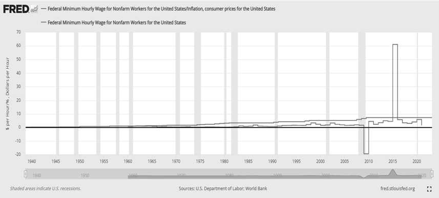
Nominal and Real Minimum Wages from 1938-2023 (2)
Minimum Wages by Change in GDP and Political Orientation (2)
VIII. Notes
- The 2SLS regressions used by Autor et al (2016) were instrumented by the log of the minimum wage, the square of the log of the minimum wage, and the log of the minimum wage interacted with the median minimum wage across states (68).
- It should be noted that Japan’s national minimum wage is indexed to the regional cost of living, and is thus not like other minimum wages (Kawaguchi and Mori 2021, 389)
- See pp. 10-11 for definitions of ‘Red State’ and ‘Blue State’ as used in the descriptive statistics in Tables 1-3.
- There are three independent senators as of 2023. Based on the author’s discretion, Senators Angus S. King Jr. of Maine, Kyrsten Sinema of Arizona, and Bernard Sanders of Vermont have been considered as ‘Democratic’—seeing as all three continue to caucus with the Democratic Party.
- For example, if a state has a minimum wage of $10, and since the federal minimum wage is $7.25, MWP would take a value equal to ln(10-7.25).
- This is by taking all states with minimum wages of $7.25, and replacing the value of the minimum wage with $7.250001, so that the end result is ln(0.000001).