Volume 35: Paper 6

An Economic Growth Comparison Between Brazil and Venezuela: An Analysis Through the Solow Growth Model

Isabella Thomas
University of Connecticut, 2025
isabella.2.thomas@uconn.edu

Dr. Natalia Smirnova
University of Connecticut
natalia.smirnova@uconn.edu

 

Understanding why some nations prosper while others falter is a central question in economics. To move beyond simple observation, growth models are often used to isolate the key drivers of national output. The Solow Growth Model is a fundamental tool in this field, providing a framework for examining how economic output is generated through capital accumulation, labor, and productivity growth. The model therefore offers a useful lens for comparative analysis across countries.

This report applies the Solow Growth Model to the sharply contrasting economic trajectories of Brazil and Venezuela. These two Latin American nations provide a compelling case study in how resource affluence can lead to vastly different outcomes. Brazil, the region’s largest economy, pursued a path of economic diversification, building major industries in agriculture, manufacturing, and services that created a more resilient economic base. Conversely, Venezuela, which possesses the world’s largest proven crude oil reserves, experienced periods of oil-fueled prosperity but ultimately suffered a severe economic collapse stemming from state mismanagement and political instability. This paper argues that Brazil’s long-run economic growth follows the predictions of the Solow growth model, where increases in capital accumulation and productivity are positively associated with GDP per capita growth, while Venezuela’s experience diverges from the model due to institutional instability and declining productivity.

 

I. Literature Review

The foundational structure for this comparative analysis is the Solow-Swan Growth Model. This framework asserts that long-run growth in output per worker is driven by exogenous technological progress, represented by Total Factor Productivity (TFP). The model established that economies converge toward a steady-state equilibrium determined by structural factors, such as the rate of saving/investment, population growth, and depreciation. In the absence of sustained TFP growth, capital accumulation alone leads to diminishing marginal returns, implying that once a country reaches its unique steady-state, per capita growth ceases. This basis is essential for evaluating whether the contrasting outcomes of Brazil and Venezuela stem primarily from differences in capital accumulation from variances in TFP, which reflects institutional quality, policy efficiency, and technological adoption.

Brazil’s growth trajectory is characterized by periods of high volatility, structural reforms, and eventual diversification. The literature on Brazil frequently highlights the institutional success in stabilizing high inflation, particularly through the implementation of the “Plano Real” (Banco Central do Brasil 2025). This monetary policy intervention served as a necessary precondition for sustained capital investment and economic planning. Earlier literature, such as that addressing the Latin American Debt Crises of the 1980s, underscores the critical role of external debt and import-substitution policies in limiting potential growth (Romero 2025). Brazil’s post-stabilization success is often attributed to its transition away from a single-commodity dependence toward a resilient structure of diverse manufacturing, service, and agricultural sectors, acting as a buffer against volatility.

The history is reflected in several distinct periods. An initial period of steady growth was driven by the implementation of an Import Substitution Industrialization (ISI) development strategy, which aimed to reduce dependency on foreign manufactured goods (Bussel 2025). Following this, the “Brazilian Miracle” from the late 1960s to 1980 saw heavy government investment in infrastructure and industries like steel and automotive manufacturing (Skidmore 2025). This growth halted during “The Lost Decade” (1980s-1990s), a period of economic instability resulting from the Latin American debt crisis. Rising global interest rates made it difficult for Brazil to service its foreign debt, and the government’s response of printing money led to hyperinflation. Subsequent growth in the 2000s was fueled by a global commodity boom, particularly demand from China (Carlson 2025). However, a recession began around 2014 as China’s economy slowed, compounded by a massive corruption scandal known as “Operation Car Wash” (Vartanian 2025).

In contrast, Venezuela’s economic history is an example of the resource curse phenomenon. Its structural decay is attributed to its overwhelming dependence on crude oil exports (Heckel et al. 2025). While oil wealth initially fueled high per capital GDP, this resilience led to a crowding out of non-oil tradable sectors and the prevention of economic diversification. From the 1950s to 1970s, Venezuela’s prosperity was fueled by its oil reserves, with the government pursuing import-substitution policies (Heckel et al. 2025). Like Brazil, Venezuela also suffered during “The Last Decade” with economic volatility (Romero et al. 2025).

Institutional factors such as fiscal mismanagement and political instability accelerated the economic collapse (Hetland 2025). A sharp increase in GDP from roughly 2003 to 2012 occurred under the administration of Hugo Chávez (Hetland 2025). This expansion was driven by high oil prices and marked by nationalizations of key industries. The nationalization policies and state control of PDVSA resulted in a severe decline in capital maintenance and oil production capacity (Muci 2024). The collapse from 2013 onward was triggered by a drop in oil prices, but its severity was due to years of misalignment that had destroyed the nation’s oil production capacity, meaning Venezuela could not benefit from future price recoveries (Muci 2024).

While the existing literature provides an institutional explanation for each country, there is a gap in studies that use a formal growth framework to directly and quantitatively contrast the two. This report seeks to fill this gap by looking into whether the growth rate of real GDP of Brazil is equal to the growth rate of real GDP of Venezuela and further decomposing the growth of both nations from 1954 to 2019 into the Solow components such as capital and labor to pinpoint which factors account for their performance.

 

II. Data & METHODOLOGY

A. Data

The datasets used in this study were obtained from the “Penn World Tables” from the Center for International Data, a credible source known for real national accounts data. The national accounts for each country are adjusted to a common currency (U.S. dollars) to allow for comparisons. It contains information about the populations, capital stock, and real GDP- this information will attribute to the Solow Growth model, which is what will be used to measure the growth for Brazil and Venezuela. The data selected is from 1954 to 2019 to capture the full cycle of the growth trajectories of both economies.

The variables selected for this analysis align with the components of the Solow Growth Model, which states that economic growth is driven by capital accumulation, labor force growth, and technological progress. Output-side real GDP (RGDPO) is utilized as the primary measure of economic output. The capital stock is proxied by capital services (RKNA). The labor force is measured using both population and (POP) and number of persons engaged (EMP). Total Factor Productivity (RTFPNA) is included to represent technological progress or efficiency. Outcome variables, such as GDP growth rate (GDPGR) and per-capita metrics for output (RGDPO/POP) and capital (RKNA/POP) are included to analyze living standards and capital intensity.

Table 1. Descriptive Statistics, Brazil

Variables	Description	Units	Mean	Minimum	Maximum	Observations
RGDPO	Output-side Real GDP at chained PPPs	mil 2017US$	1232958.120	113028.422	3306056.000	66
RKNA	Capital services at constant 2017 national prices	Index(2017=1)	0.427	0.045	1.022	66
POP	Population	mil persons	137.736	59.631	211.050	66
EMP	Number of persons engaged	mil persons	54.024	18.987	93.957	66
RTFPNA	TFP at constant national prices	Index(2017=1)	1.184	0.874	1.547	66
GDPGR	GDP Growth Rate	Percentage change from previous year	0.054	-0.065	0.201	65
RKNA/POP	Capital Services per Capita	2017 US$ per person	0.003	0.001	0.005	66
RGDPO/POP	GDP per Capita	2017 US$ per person	7542.349	1895.457	16611.414	66

Source: PWT version 10.01, n.d. “File PWT 1001. Data for Brazil 1954 and 2019.” University of Groningen.

 

Table 2. Descriptive Statistics, Venezuela

Variables	Description	Units	Mean	Minimum	Maximum	Observations
RGDPO	Output-side Real GDP at chained PPPs	mil 2017US$	184613.937	7160.107	615473.438	66
RKNA	Capital services at constant 2017 national prices	Index(2017=1)	0.558	0.098	1.101	66
POP	Population	mil persons	18.334	6.270	30.082	66
EMP	Number of persons engaged	mil persons	6.554	1.921	12.978	66
RTFPNA	TFP at constant national prices	Index(2017=1)	2.026	0.567	3.175	66
GDPGR	GDP Growth Rate	Percentage change from previous year	0.000	-0.799	0.284	65
RKNA/POP	Capital Services per Capita	2017 US$ per person	0.028	0.016	0.037	66
RGDPO/POP	GDP per Person	2017 US$ per person	9797.146	251.092	20962.394	66

Source: PWT version 10.01, n.d. “File PWT 1001. Data for Venezuela 1954 and 2019.” University of Groningen.

The descriptive statistics from Tables 1 and 2 reveal significant structural differences between the two economies. Brazil, on average, possesses a much larger economy, with a mean real GDP of $1.23 trillion, significantly exceeding Venezuela’s mean of $184.6 billion. This is consistent with its labor force metrics, where Brazil’s mean population and engaged persons are roughly 7.5 and 8.2 times larger than Venezuela’s, respectively. However, their per-capita metrics illustrate a different economic relationship. Venezuela’s mean GDP per capita is higher at $9,797.15, compared to Brazil’s $7,542.35, suggesting a higher measured average income or output per person. This is strongly correlated with its higher mean capital services per capita, which is more than ten times than that of Brazil. This distinction highlights Venezuela’s economic structure as a capital-intensive petrostate. Conversely, Brazil’s economy appears to be driven more by its large labor factor than by capital intensity. Of note is the extreme volatility in Venezuela’s variables, especially the GDP growth rate, which has a minimum of -79.9 percent and a mean near 0. This indicates a catastrophic economic collapse for Venezuela. Brazil’s growth, while also variable, has been more stable and consistently positive on average. This suggests that while Venezuela’s resource concentration may have enabled periods of higher per-capita income, it also introduced extreme instability, whereas Brazil’s growth has been more grounded in labor accumulation.

 

B. Method 1: Trend Analysis

Figure 1. Real GDP Trend, Brazil, 1954-2019

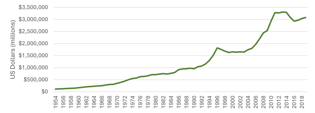
Source: PWT version 10.01, n.d. “File PWT 1001. Data for Brazil 1954 and 2019.” University of Groningen.

 

Figure 2. Real GDP Trend, Venezuela, 1954-2019

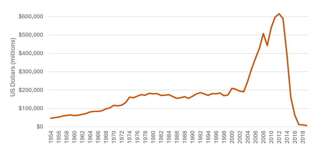
Source: PWT version 10.01, n.d. “File PWT 1001. Data for Venezuela 1954 and 2019.” University of Groningen.

 

Figure 3. Comparisons of GDP Growth Rates Between Brazil and Venezuela, 1954-2019

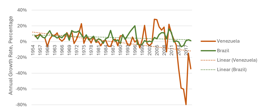
Source: PWT version 10.01, n.d. “File PWT 1001. Data for Brazil and Venezuela 1954 and 2019.” University of Groningen.

 

Figure 4. Production Function, Brazil

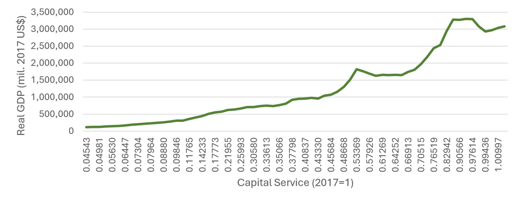
Source: PWT version 10.01, n.d. “File PWT 1001. Data for Brazil 1954 and 2019.” University of Groningen.

 

Figure 5. Production Function, Venezuela

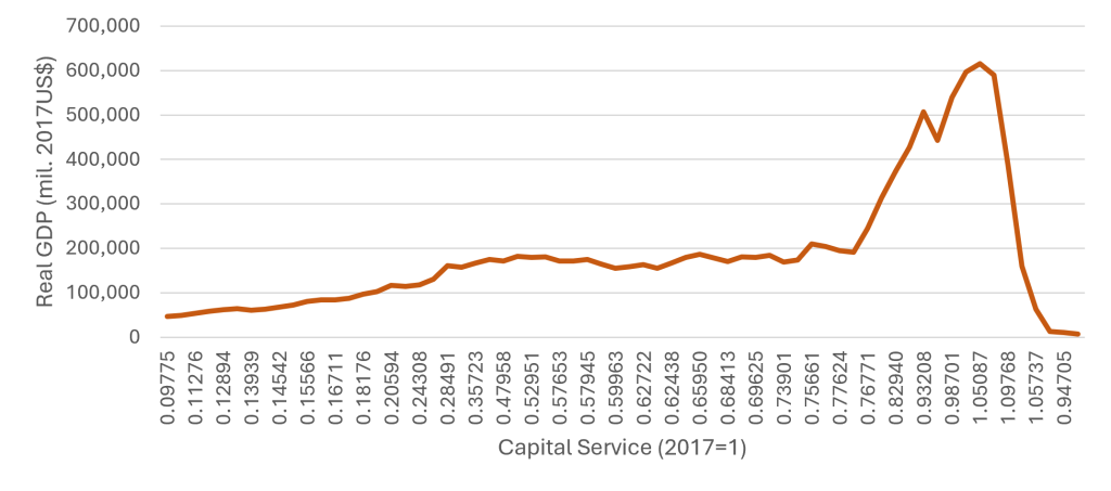
Source: PWT version 10.01, n.d. “File PWT 1001. Data for Venezuela 1954 and 2019.” University of Groningen.

 

Figure 6. Labor Trend, Brazil

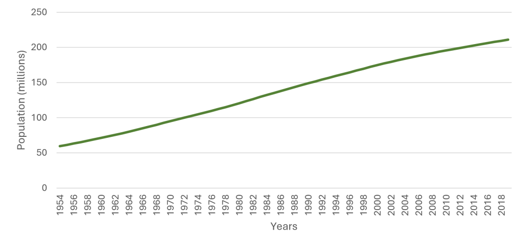
Source: PWT version 10.01, n.d. “File PWT 1001. Data for Brazil 1954 and 2019.” University of Groningen.

 

Figure 7. Labor Trend, Venezuela

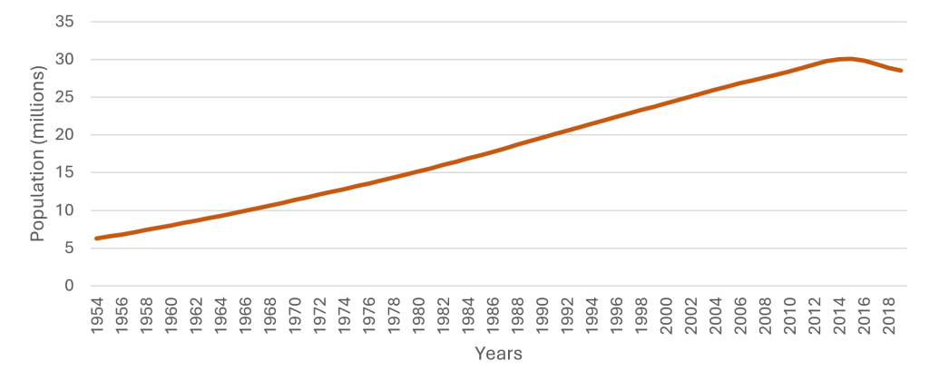
Source: PWT version 10.01, n.d. “File PWT 1001. Data for Venezuela 1954 and 2019.” University of Groningen.

 

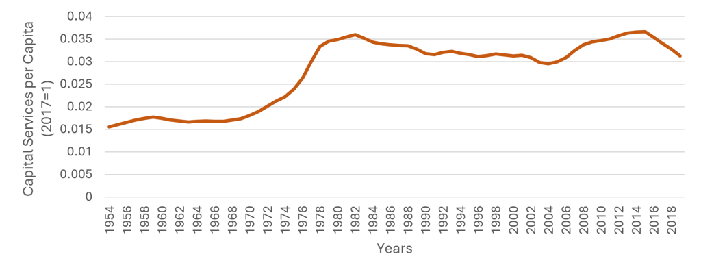
Figure 8. Capital per Capita Trend, Brazil

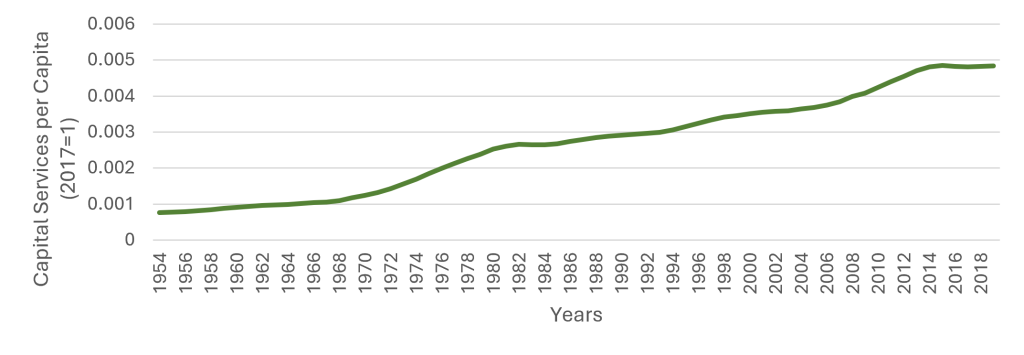
Source: PWT version 10.01, n.d. “File PWT 1001. Data for Brazil 1954 and 2019.” University of Groningen.

 

Figure 9. Capital per Capita Trend, Venezuela

Source: PWT version 10.01, n.d. “File PWT 1001. Data for Venezuela 1954 and 2019.” University of Groningen.

 

Figure 10. TFP, Brazil

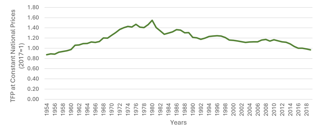
Source: PWT version 10.01, n.d. “File PWT 1001. Data for Brazil 1954 and 2019.” University of Groningen.

 

Figure 11. TFP, Venezuela

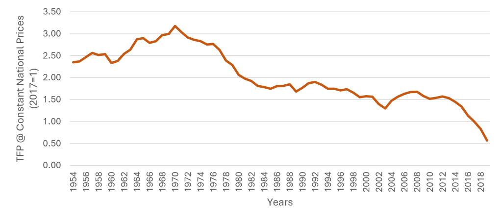
Source: PWT version 10.01, n.d. “File PWT 1001. Data for Brazil 1954 and 2019.” University of Groningen.

C. Method 2: Data Regression

This study employs a multiple linear regression model based on the Solow Growth framework to examine the determinants of economic growth in Brazil and Venezuela from 1954 to 2019. The Solow model states that economic growth is driven by capital accumulation, labor force growth, and technological progress. As a result, the analysis focuses on estimating the relationship between real GDP per capita growth and other key variables. The dependent variable in this study is the annual growth rate of real GDP per capita, calculated as the ratio of Output-side real GDP (RGDPO) to population (POP). The three independent variables are the following: capital per capita (RKNA/POP), TFP at constant national prices (RTFPNA), and employment (EMP) representing labor force. The observed independent variable will be the capital per capita. All variables are transformed into logarithms, linearizing exponential growth relationships, and further allowing for direct interpretation of coefficients. The regression equation will be expressed as the following:

(1) Δln(Y_t) = β_{0 +} β₁(ln(RKNA/POP)_t) + β₂(ln(RTFPNA)_t) + β₃(ln(EMP)_t) + u_t

The hypotheses created from this study are null and alternative. The null hypothesis states there is no significant difference in the factors contributing to real GDP per capita growth between Brazil and Venezuela. The alternative hypothesis states that there are in fact significant differences between the effects of capital per person, total factor productivity, and labor force on real GDP per capita growth between Brazil and Venezuela.

Table 3. Regression Output Table, Brazil

	Coefficients	Standard Error	t Stat	P-value
Intercept	15.073	0.168	89.577	0.000
Growth Rate Capital per Person	1.040	0.028	37.780	0.000

Source: PWT version 10.01, n.d. “File PWT 1001. Data for Brazil 1954 and 2019.” University of Groningen.

 

Figure 12. Residual Plot, Brazil

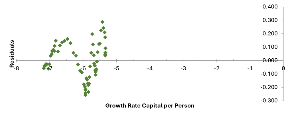
Source: PWT version 10.01, n.d. “File PWT 1001. Data for Brazil 1954 and 2019.” University of Groningen.

 

Table 4. Regression Output Table, Venezuela

	Coefficients	Standard Error	t Stat	P-value
Intercept	8.813	1.172	7.517	0.000
Growth Rate Capital per Person	-0.059	0.323	-0.183	0.856

Source: PWT version 10.01, n.d. “File PWT 1001. Data for Venezuela 1954 and 2019.” University of Groningen.

 

Figure 13. Residual Plot, Venezuela

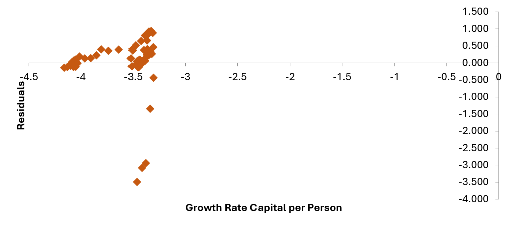
Source: PWT version 10.01, n.d. “File PWT 1001. Data for Venezuela 1954 and 2019.” University of Groningen.

III: Analysis

A. Method 1: Trend Analysis

1. Real GDP Trend

Figure 1 for Brazil’s real GDP trend from 1954 to 2019 can be segmented into four distinct periods. 1954 to 1980 represents a period of steady, consistent upward growth, with real GDP rising from approximately $113 billion to over $750 billion. 1980 to 1994 is a period of volatility and stagnation, where growth halted and fluctuated, showing little net increase over more than a decade. 1994 to 2014 represents a phase of sharp, accelerated growth. Real GDP rises steeply from approximately $1.25 billion to a peak of approximately $3.3 trillion. 2014 to 2019 marks the final period showing a sharp recession, with real GDP falling from its peak, followed by a slow recovery by 2019.

Figure 2 illustrates Venezuela’s real GDP trend from 1954 to 2019, which is also marked by four distinct phases. 1954 to 1980 marks a period of a steady upward climb, with GDP rising from under $50 billion to approximately $175 billion. 1980 to 2003 represents a long period of high volatility and stagnation, with GDP struggling to regain its previous peak, fluctuating between $150 billion and $200 billion. 2003 to 2012 is a period of extremely rapid expansion, with GDP surging from its stagnant level to a peak of over $600 billion. The period from 2013 to 2019 represents a catastrophic economic collapse. The figure shows a near-vertical decline, with the nation’s real GDP falling from its peak to below $50 billion, erasing decades of economic accumulation.

2. Comparisons of GDP Growth Rate

Figure 3 plots the annual growth rates of both Venezuela’s and Brazil’s economies. Prior to the 21^st century, both nations experienced significant economic volatility, reflected in frequent and drastic fluctuations in growth. Brazil and Venezuela’s growth often move in opposing directions, but both show periods of high positive growth offset by years of stagnation and recession. The post-2000 period, however, marks a significant divergence. Brazil’s growth rate, while still variable, shows a positive trend from the early 2000s until around 2012 (Carlson et al. 2025). Venezuela’s trajectory presents a stark contrast. After its own period of high growth, it reveals a devastating decline, with annual growth rates plummeting to catastrophic negative levels after 2014, reversing decades of economic progress.

3. Production Function

In Figures 4 and 5, capital services are indexed so that 2017 = 1. Every other observation is a ratio to that base year. Brazil’s production function in Figure 4 is upward sloping but non-linear. It displays a slow rise at low capital intensity, which then gives way to a sharper increase in GDP as capital services increase. At the higher levels (approaching 1.0), the function begins to flatten and decrease, suggesting that Brazil is reaching the limits of capital accumulation, thus signaling diminishing returns.

Venezuela’s production function in Figure 5 has undergone a severe collapse. From 1954 until its peak, the function shows a positive relationship where increases in capital services were associated with an increase in real GDP, peaking at over $600 billion. However, the rightmost portion of the graph shows a complete structural failure. As capital services peaked and declined from their maximum of approximately 1.05087, real GDP collapsed. This indicates a failure of the productive structure, rendering much of the existing capital virtually useless.

4. Labor Trend

Figure 6 demonstrates that the population of Brazil is sustaining positive growth throughout 1954 to 2019. The continuous upward trajectory shows Brazil had an expanding human resource base to feed the working-age population throughout the period, making labor factor growth a consistent contributor to the nation’s potential GDP growth. However, sometime after 2010, the line begins to curve slightly, signaling a deceleration in the growth rate.

Venezuela’s labor trend in Figure 7 shows an increase in population from 1954 to roughly 2008, where it then begins to curve and decline in 2014. This is a visual indicator of massive emigration driven by the severe economic and political crisis, which constitutes a significant and active erosion of the country’s labor force input, acting as another constrain on Venezuela’s long-run potential GDP growth (Muci 2024).

5. Capital per Capita Trend

As shown in Figure 8, from 1954 to 1970, Brazil’s capital per capita trend experiences slow growth, followed by a phase of accelerated capital accumulation, reflecting high investment that raised capital per person. However, upon reaching “The Lost Decade,” the accumulation abruptly halted, thus resulting in the stagnation due to inefficient investment levels (Romero et al. 2025). While there is another increase from 1996 to 2014, it ends with a plateau, indicating a sudden halt in the growth of capital per capita. This is due to the impact of the 2014-2016 Recession, where the collapse of investment spending prevented further capital deepening (Vartanian et al. 2025).

Figure 9 documents the highly unstable evolution of Venezuela’s capital per capita. The period from 1954 to 1982 was marked by robust capital deepening, as shown by the steep, continuous increase in capital per worker, particularly between 1972 and 1982. This suggests that gross investments significantly outpaced the required break-even investment, allowing the economy to increase its productive capacity. However, this expansion gave way to two decades of instability and stagnation, where the K/L ratio declined from its peak and fluctuated. This implies that national saving and investment levels were inadequate to sustain capital deepening, resulting in no net increase in output per worker and thus limiting Venezuela’s potential for sustainable real GDP growth. The final segment highlights an economically devastating structural collapse. After a short, unstable recovery, the K/L ratio reached a final peak around 2014 before entering a sharp decline through 2018. This drop signals a severe erosion of the nation’s capital stock (Muci 2024).

6. TFP

In Figure 10, Brazil’s initial phase, spanning the 1950s to 1980, shows a period of upward growth. During this time, the TFP would move consistently above the 1.0 base index, eventually reaching its peak around the 1.55 maximum established in the descriptive data in Table 1. However, the second phase, likely beginning with the “Lost Decade” of the 1980s and extending through recent times, shows a marked shift towards volatility and stagnation. This is characterized by the sharp drop in TFP, eventually touching the 0.87 minimum. While the economy expanded in size, its efficiency struggled to consistently move beyond past peaks.

In Figure 11, throughout the period, Venezuela’s TFP index ranged from a minimum of 0.57 to a maximum of 3.17 reached around 1970, as stated in the descriptive data in Table 2. Following the initial peak, the TFP index begins with a persistent decline, characterized by a series of sharp drops. Throughout the 1980s and 1990s, the index attempts several upward corrections but fails to achieve any sustained growth, remaining structurally below the initial period’s levels. The most critical feature is the movement starting in the late 1990s, where the index enters a terminal, steep decline, eventually dragging the TFP index to its minimum of 0.57. Visually, the graph demonstrates an economy that experienced an early boom followed by decades of consistent erosion of its productive efficiency, resulting in a non-recovering structural failure (Hetland 2025; Muci 2024).

 

B. Method 2: Data Regression

For Brazil, the regression model yields a coefficient of 1.0399 for the “Growth Rate Capital per Person” (ln(rkna/pop)) variable as seen in Table 3. This coefficient suggests that, within this model, a 1 percent increase in the growth rate of capital per person is associated with an approximate 1.04 percent increase in the growth rate of real GDP per capita. The p-value of this coefficient is approximately 0.000, therefore the null hypothesis is rejected, concluding that the growth rate of capital per person is a significant predictor of real GDP per capita growth in Brazil. The model’s explanatory power is high, with an R² of 0.957, indicating that 95.70 percent of the variation in Brazil’s per capital GDP growth is explained by the growth in its capital per person.

However, the residual plot in Figure 12 reveals an issue within the model specification. The residuals are not randomly scattered but instead display a distinct fanning or U-shaped pattern. This pattern indicates the presence of heteroskedasticity, meaning the variance of the error terms is not constant across observations. This implies that, while the overall relationship may appear strong, the estimated standard errors are biased, rendering the results- including the t-statistics and p-values- unreliable.

The model for Venezuela provides a stark contrast. In Table 4, the coefficient for the “Growth Rate Capital per Person” variable is –0.0589, suggesting a negative relationship and implying capital accumulation is not associated with positive growth. Given the coefficient’s p-value of approximately 0.8556, the null hypothesis fails to be rejected, and it must be concluded that there is no statistical evidence of a relationship between the growth of capital per person and the growth of real GDP per capita in Venezuela. The model’s explanatory power confirms this lack of relationship. The R² is 0.001, indicating that the model explains 0.05 percent of the variation in Venezuela’s per capita GDP growth.

The residual plot in Figure 13 displays a distinct “cone-shaped” distribution, indicating severe heteroskedasticity. This suggests that the variance of the residuals increases systematically with the level of capital growth. Combined with the statistically insignificant p-value and near zero R², this confirms that the model provides no meaningful explanatory power for Venezuela’s economic growth. Additional regression output and diagnostic results are provided in the Appendix.

 

IV. Conclusion

The central research question was whether the growth rates of the two nations were equal and further looking into which Solow components account for their performance. Given this analysis, the answer is a definitive no. The trend analysis showed Brazil achieved long-term growth rooted in labor force expansion and capital accumulation, while Venezuela experienced a complete economic collapse driven by institutional failure and a decreasing labor force. The regression analysis confirmed this divergence: while flawed, Brazil’s growth showed a high correlation with capital, while Venezuela showed no statistically significant relationship with the growth of its capital per person. This lack of explanatory power in the Venezuelan model strongly suggests its economic collapse is driven by factors outside of this capital-based framework, such as the decline in TFP and institutional failures noted in the literature review.

 

A. Limitations

While conducting this study, there were a few limitations. One was the use of simple regression, where only one independent variable was used. This resulted in omitted variable bias, as factors such as TFP were not included. Another was patterns of heteroskedasticity shown in both residual plots for Brazil and Venezuela. This violation of OLS assumptions means that the standard errors and p-values are unreliable. A further limitation was the use of population (pop) as the denominator for per-capita metrics, rather than the number of persons engaged (emp). This choice, while useful for a broad measure of national prosperity, is less precise for measuring the ‘per worker’ components central to the Solow model’s production function. Ultimately, instead of using capital stock, capital services (rkna) was used as a proxy. This may not have fully captured the productive capacity of capital, especially in Venezuela, where capital may exist but be non-operational.

B. Avenues for Future Research

This report quantitively confirms that Brazil’s economy, while struggling with its own TFP stagnation, operates on an economic framework where capital accumulation drives growth. Venezuela, however, does not. It is a case of state-driven institutional collapse where standard economic inputs no longer function predictably. Future research is essential to build upon these findings. A necessary first step is to correct this study’s limitations by developing a multiple regression model that incorporates the omitted variables. This model must also be corrected for heteroskedasticity by using robust standard errors to produce reliable t-statistics. A more focused study could also attempt to decompose the TFP collapse in Venezuela, possibly using a qualitative analysis to pinpoint the specific impacts such as those of nationalization and price controls on productive efficiency. Further, there can be a comparative case study focusing on specific policy decisions, such as Brazil’s “Plano Real” versus Venezuela’s price controls, to qualitatively assess their direct impact on TFP and investment.

C. Policy Recommendations

Based on these findings, the policy paths for each nation are starkly different. For Brazil to overcome its stagnation, policies must focus on boosting TFP through education and research and development and maintaining the fiscal stability established by the “Plano Real.” Further, institutional reform to tackle corruption and improve the regulatory environment is advised. Venezuela’s economy requires stabilization and fundamental institutional restoration. This requires immediate macroeconomic stabilization to halt hyperinflation and a massive effort to attract foreign investment to rebuild the nation’s collapsed oil capacity. Concurrently, Venezuela must implement policies to reverse its emigration to restore its labor force and, once, stable, create a long-term framework to break the “resource curse.”

This comparative analysis empirically demonstrates the profound divergence between Brazil and Venezuela. It highlights that while Brazil’s economy, though volatile, aligns with the Solow framework’s emphasis on capital accumulation, Venezuela’s trajectory does not. This study ultimately underscores how sound policy and institutional stability are the fundamental preconditions for economic inputs, such as capital and labor, to generate national prosperity.

 

Appendix

 

Table A1. (Complete) Regression Output Table, Brazil

	Coefficients	Standard Error	t Stat	P-value	Lower 95 Percent	Upper 95 Percent	Lower 95.0 Percent	Upper 95.0 Percent
Intercept	15.073	0.168	89.577	0.000	14.736	15.409	14.736	15.409
Growth Rate Capital per Person	1.040	0.028	37.780	0.000	0.985	1.095	0.985	1.095

Source: PWT version 10.01, n.d. “File PWT 1001. Data for Brazil 1954 and 2019.” University of Groningen.

 

Regression Statistics, Brazil

Multiple R	0.978
R Square	0.957
Adjusted R Square	0.956
Standard Error	0.133
Observations	66

Source: PWT version 10.01, n.d. “File PWT 1001. Data for Brazil 1954 and 2019.” University of Groningen.

 

Residual Output (first 15), Brazil

Observation	Predicted Y	Residuals
1	7.606	-0.059
2	7.630	-0.039
3	7.640	-0.042
4	7.678	-0.026
5	7.706	-0.027
6	7.754	-0.060
7	7.785	-0.028
8	7.822	0.035
9	7.853	0.048
10	7.867	0.072
11	7.882	0.071
12	7.905	0.080
13	7.934	0.070
14	7.949	0.109
15	7.982	0.147

Source: PWT version 10.01, n.d. “File PWT 1001. Data for Brazil 1954 and 2019.” University of Groningen.

Table A2. (Complete) Regression Output Table, Venezuela

	Coefficients	Standard Error	t Stat	P-value	Lower 95 Percent	Upper 95 Percent	Lower 95.0 Percent	Upper 95.0 Percent
Intercept	8.813	1.172	7.517	0.000	6.471	11.155	6.471	11.155
Growth Rate Capital per Person	-0.059	0.323	-0.183	0.856	-0.704	0.586	-0.704	0.586

Source: PWT version 10.01, n.d. “File PWT 1001. Data for Venezuela 1954 and 2019.” University of Groningen.

 

Regression Statistics, Venezuela

Multiple R	0.022819412
R Square	0.000520726
Adjusted R Square	-0.015096138
Standard Error	0.784311991
Observations	66

Source: PWT version 10.01, n.d. “File PWT 1001. Data for Venezuela 1954 and 2019.” University of Groningen.

 

Residual Output (first 15), Venezuela

Observation	Predicted Y	Residuals
1	9.058	-0.142
2	9.057	-0.119
3	9.055	-0.083
4	9.053	-0.031
5	9.052	-0.016
6	9.051	-0.008
7	9.052	-0.110
8	9.053	-0.116
9	9.054	-0.081
10	9.055	-0.046
11	9.054	0.024
12	9.054	0.024
13	9.054	-0.005
14	9.054	-0.004
15	9.053	0.072

Source: PWT version 10.01, n.d. “File PWT 1001. Data for Venezuela 1954 and 2019.” University of Groningen.

 

References

2025. Brazil’s Productivity Challenge: Structural Change versus Economy-Wide Innovation-Based Improvements in: Brazil. https://www.elibrary.imf.org/display/book/9781484339749/ch004.xml.

Bussel, Jeniffer. 2025. “Import Substitution Industrialization.” Encyclopædia Britannica. Encyclopædia Britannica, inc. https://www.britannica.com/money/import-substitution-industrialization.

Carlson, Eric, and Ravi Jain. 2025. “Brazil: Rewiring the Economy.” Morgan Stanley Investment Management. https://www.morganstanley.com/im/en-us/individual-investor/insights/tales-from-the-emerging-world/brazil-rewiring-the-economy.html.

Heckel, Heather, McCoy, Jennifer, et al. 2025. “Economy of Venezuela.” Encyclopædia Britannica. Encyclopædia Britannica, inc. October 5. https://www.britannica.com/place/Venezuela/Economy.

Hetland, Gabriel. 2025. “Is Hugo Chávez to Blame for Venezuela’s Collapse?” North American Congress on Latin America (NACLA). June 24. https://nacla.org/is-hugo-chavez-to-blame-for-venezuelas-collapse/.

Muci, Frank. 2024. “Why Did Venezuela’s Economy Collapse?” Economics Observatory. September 24. https://www.economicsobservatory.com/why-did-venezuelas-economy-collapse.

“PWT 10.01.” 2024. University of Groningen. November 18. https://www.rug.nl/ggdc/productivity/pwt/.

Ravikumar, B., and Dawn Chinagorom-Abiakalam. 2024. “Convergence or Divergence? A Look at GDP Growth across Richer and Poorer Countries.” https://www.stlouisfed.org/on-the-economy/2024/aug/convergence-divergence-gdp-growth-richer-poorer-countries

Banco Central Do Brasil. 2025.“The Real Plan.” https://www.bcb.gov.br/en/monetarypolicy/realplan.

Romero, Jocelyn Sims and Jessie. 2025. “Latin American Debt Crisis of the 1980s.” Federal Reserve History. https://www.federalreservehistory.org/essays/latin-american-debt-crisis.

Skidmore, Thomas. 2025. Brazil Five Centuries of Change. https://library.brown.edu/create/fivecenturiesofchange/chapters/chapter-7/economic-miracle/.

Vartanian, Pedro, and Hugo de Souza Garbe. 2025. The Brazilian Economic Crisis during the Period 2014-2016. https://www.mackenzie.br/fileadmin/ARQUIVOS/Public/6-pos-graduacao/upm-higienopolis/mestrado-doutorado/economia_mercados/2020/Anais_de_Congresso/The_Brazilian_economic_crisis_during_the_period_2014-2016.pdf.