Volume 32, Issue 1: Paper 2

Can Workfare Increase Ownership of Productive Assets?

Evidence from India’s National Rural Employment Guarantee Scheme

Hugh O’Reilly University of Manchester

The National Rural Employment Guarantee Scheme (NREGS) is one of the largest social protection schemes to ever exist, and is certainly the largest workfare programme, providing employment to between 21 and 55 million households every year since its inception in 2006 (Reddy, Roy and Pradeep, 2021). The 2005 Mahatma Gandhi National Rural Employment Guarantee Act (MGNREGA), upon which the scheme was enacted, made employment a legal right for rural adults, and aimed to provide at least 100 days of work to those who choose to participate, in an eﬀort to ensure employment opportunities for the poorest whilst improving infrastructure at a local level. Unemployment allowances are distributed where demand for work cannot be met. The majority of work under the scheme is used to increase agricultural productivity by constructing and improving irrigation systems, roads, water access, environmental conservation, extreme weather-proofing and general land development (Ministry of Rural Development, 2013). Public works have been part of Indian policy discourse for millennia, with the first documented advocate of their use being ancient Indian polymath and royal advisor Chanakya (Dreze and Sen, 1990). Other large public work programmes in developing countries include Bangladesh’s Food-For-Work (FFW) programme and Ethiopia’s Productive Safety Net Programme (PSNP), with their popularity increasing in response to the COVID-19 pandemic (Gentilini et al., 2020).

Given the size of the scheme, which accounts for 1.5-4 percent of annual government expenditure (Ehmke, 2015), and the decentralised manner in which it has been implemented, the impacts experienced across the nation have been varied. As a whole, minority groups within India (women, Scheduled Castes and Scheduled Tribes) account for a larger share of participants than they do in the labour force (Haque, 2011). This additional employment option has reduced the dependency of such groups on land-owners who control local monopsonies in agriculture. Furthermore, the scheme increased market equilibrium wages for low-skill labour (Imbert and Papp, 2015; Berg et al., 2018), particularly for women (Azam, 2011; Zimmerman, 2012). A study by Bose (2017) concluded that the scheme increased rural household consumption expenditure by 6.5-10 percent, whilst Ravi and Engler (2009) found that in Andhra Pradesh food security improved, with participants experiencing less anxiety and having a higher probability to save. These welfare eﬀects occurred particularly during the agricultural oﬀ-season (Klonner and Oldiges, 2022). Further benefits occurred from the projects themselves, which caused an increase (albeit small) in agricultural productivity in West Bengal (Kundu and Talukdar, 2016), with 90 percent of respondents in Ranaware et al. (2015) considering the works very useful or somewhat useful. Many works addressed the depletion of natural resources, and reduced vulnerability to long-term climate risks (Esteves et al. 2013). All of these outcomes have poverty-reducing eﬀects. However, the scheme does not exist without flaws. For years, it has received criticism for its inability to meet demand; in 2009/2010, 44.7 percent of all households who applied for work did not receive any (Dutta et al., 2012). Furthermore, delayed payments to participants in the NREGS is common, an issue worsened by the leakage of funds due to corrupt practices, such as the over-reporting of work by public oﬃcials (as evidenced in Imbert and Papp [2011]). Perhaps most concerning is the steady decline of project completion rates from 47 percent in 2006/2007 to just 18 percent in 2017/2018 (Reddy, Roy and Pradeep, 2021). This represents an increasingly large waste of resources, which reduces the benefits for local communities and brings into question whether an unconditional cash transfer could be more eﬀective, as suggested by Alik-Lagrange and Ravallion (2018).

Clearly, the evidence of the scheme’s success is mixed. Given that the pioneering NREGS is an influential model for workfare programmes across the world, further impact evaluation is needed, particularly regarding the mechanisms in which the scheme insures against shocks and encourages growth in real living standards. This paper will contribute to the ongoing welfare assessment of the NREGS from a relatively neglected perspective; the eﬀect of participation on household’s productive asset holdings. Specifically, this research will examine assets that are deemed to have returns through time, eﬀort and attention saving properties, as well as assets that provide income-generating opportunities.

There are several reasons why investigating the scheme’s impact on household productive asset ownership is of interest for policymakers. Household assets intrinsically provide individuals the capability to perform basic tasks that are essential to achieving well-being/happiness, whereby the failure of “certain basic capabilities” (Sen, 2006, p. 34) is the fundamental nature of poverty. Therefore, programmes which aﬀect asset accumulation will also aﬀect levels of poverty – a top priority for global governance, most notably formalised by ‘Goal 1’ of the United Nations’ Sustainable Development Goals (2022). The notion that asset holdings determine poverty is strengthened by theoretical work from Banerjee and Mullainathan (2008), who assert that poor households allocate more attention to domestic matters since they lack “distraction-saving goods and services” (p. 489). Therefore, they are unable to maximise their marginal product of labour (and sub- sequent wage) in the labour market, establishing a vicious cycle of persistent poverty. Consequently, policy which can increase asset ownership may increase economic participation and labour productivity in the long run. Furthermore, dissaving and the sale of assets is a common coping strategy of the global poor when facing an income shock (Deaton, 1989; Naudé et al., 2009). Because of this, asset holdings oﬀer crucial insight into levels of self-insurance and vulnerability (Vatsa, 2004). This should be considered alongside the conceptualisation of workfare as a direct form of insurance in itself (and therefore a substitute to selling assets), as argued by Johnson (2009) and Fetzer (2020) amongst others.

Specifically for India’s NREGS, investigating private asset outcomes is important since they determine project inclusivity and usability. This is because the social welfare returns of most local public infrastructure projects are maximised when households in the community have the private assets required to make use of them. For example, roads are most advantageous if people own vehicles, and improved irrigation systems are most beneficial if households own suﬃcient agricultural equipment to generate the intended productivity gains.

This paper proceeds as follows. In the literature review, I summarise influential research concerning workfare and the NREGS specifically, identifying previous works which oﬀer evidence on asset outcomes. Next, I describe the data using key demographic variables, with a focus on NREGS participation. I then explain and justify my empirical strategy, highlighting the main limitations. After this, I present the results, discussion and concluding remarks.

II. Literature Review

The term ‘workfare’ was first popularised by Richard Nixon as an alternative to traditional welfare policy during his presidential reforms in the early 1970s (Peck, 1998). However, as relief work in developing coun- tries evolved into longer term employment schemes, such as the Employment Guarantee Scheme (EGS) in Maharashtra (Bagchee, 1984), literature redefined workfare in the relatively new context of the rural devel- oping world. Early work by Walker, Singh and Asokan (1986) found that income variation halved for landless labourers where the EGS became available. However, more influential literature on workfare focused on the benefits of self-targeting. Besley and Coate’s (1992) theoretical analysis of a work requirement for welfare demonstrated that at an appropriate wage level the non-poor are unwilling to work since their reservation wage is not met. Following this, workfare was characterised as a pragmatic strategy for targeting the poor in the development sphere; Ravallion (1991) suggested that self-targeting of the poor makes it practical compared to alternatives, given that “means-tested transfers are rarely feasible in rural areas of developing countries” (p. 170).

Morduch (1999) oﬀers theoretical insight into the potential wealth benefits of welfare with work require- ments, hypothesising that it can reduce the need for households to dissave or sell assets when facing a shock. Ravallion (1991) goes further to suggest that “the extra insurance provided may also encourage more productive investment” (p. 171).

With that said, what existing evidence is there on the impact of workfare participation on productive household assets? A study by Berhane et al. (2014) used a diﬀerence-in-diﬀerence model with propensity score matching (PSM) to show that an extra four years of participation after the first year in Ethiopia’s PSNP caused an average increase of livestock by 0.38 units. However, given the first survey was conducted after the PSNP was implemented, the results are not able to capture the full eﬀect of participation. Empirical literature which focusses on the NREGS is more extensive. Although it’s not a definitive determinant of household assets, Ravi and Engler (2015) use a similar methodology of triple-diﬀerence estimation with PSM to show that the probability of saving is 21 percent higher for participants compared to those who applied but did not receive work. From another perspective, Varman and Kumar (2020) found that NREGS participation increased the share of monthly consumption expenditure that went towards durable goods. Despite it being statistically significant, the result was too small to hold economic relevance. Furthermore, the results are susceptible to selection bias, since they make no eﬀort to mitigate the issue of non-random treatment allocation which stems from the self-selective property of the scheme.

Arguably, the best attempts at estimating the impact of workfare participation on household asset holdings within the context of the rural developing world have been by Deininger and Liu, in 2010 and 2019. Both adopt an empirical strategy of diﬀerence-in-diﬀerence, using PSM to mitigate the eﬀects of voluntary participation. Statistically significant results from their 2010 paper find the eﬀect of participation on non-financial assets (composed of consumer durables, livestock and equipment) to range between 7.5 percent and 15.3 percent. In 2019, they found the eﬀect to be 16.4 percent. Their results support the economic intuitions of Morduch (1999) and Ravallion (1991), concluding that the increased access to non-financial assets also reduced their vulnerability to shocks. This indicates that the NREGS has two insurance eﬀects that can substitute for dissaving and the sale of assets; 1. The direct property of work as a legal entitlement, and 2. The indirect mechanism by which asset accumulation is enabled, subsequently leading to the diversification of income- generating activity.

The research by Deininger and Liu has produced results which extend the knowledge we have on workfare in the rural context of a developing country. However, as with all empirical research, it has its limitations. By restricting their sample to the state of Andhra Pradesh, the estimates are unable to represent the impact of the NREGS on non-financial assets in its entirety, since the sample is not representative at a national level. As they explain, Andhra Pradesh had a quicker, more eﬃcient implementation of the NREGS for many reasons, including long-established self-help groups for women and anti-corruption strategies which other states did not adopt as early. Further evidence that Andhra Pradesh is not representative of the entire country comes from Dutta et al. (2012), who shows that the state had the third highest programme expenditure per capita in 2009-2010 (749Rs), and the highest programme expenditure per capita in 2010-2011 (896Rs). For these reasons, Andhra Pradesh is “one of a few star performers in terms of the quality of program implementation” (Liu and Deininger, 2019, p. 100). Inherently, any results obtained from the study represent the state alone and cannot be extrapolated to the scheme as a whole.

Additionally, their estimates on asset accumulation are limited by the small time span, where post- implementation data is retrieved from 2008. Asset accumulation typically requires gradual saving over extended periods of time, yet the data can only account for the first two years of the scheme. Conse- quently, the study is unable to capture the long-run, nationwide accumulation eﬀect of the scheme as a well established source of employment in the low-skill labour market of rural India.

Given these data limitations in Deininger and Liu (2010; 2019), there is no all-inclusive evidence of the NREGS’ average participation eﬀect on household asset holdings in the long run. This paper attempts to fill the gap, using nationally representative data collected over a more extended time frame, giving policymakers improved evidence on the impacts of the NREGS and contemporary workfare as a whole.

III. Data

Data is sourced from the publicly-available Indian Human Development Survey (IHDS) series (see Table A in the appendix), which have intrinsic value for NREGS policy evaluation due to the survey timings; the first round occurred shortly before implementation (2004-2005) and the second round occurred years after full nationwide implementation (2011-2012). The series is nationally representative, containing 41554 households in the IHDS-I and 42152 households in the IHDS-II, which consists of reinterviewed households (83 percent) and a replacement sample. The data enables me to quantify the scheme’s impact for the country in its entirety, whilst also preventing sample size from being a predominant concern in statistical inference.

Figure 1

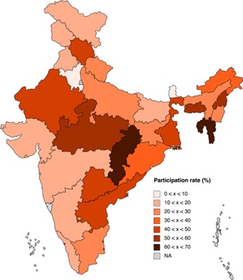
(a) NREGS participation of job card holders by state

(b) Income dependency of participants on the NREGS by state

Note: Statistics for Ladakh and Telangana are obtained from their previous union territories / states

Given the diﬀering administrative capabilities and demand for the scheme across states, implementation of the MGNREGA was varied in terms of coverage and impact (Reddy, Roy and Pradeep, 2021). Figure 1(a) shows how Eastern states in particular have performed relatively well in terms of meeting demand for the scheme, with over 50 percent of job card households (households who have applied for NREGS work) receiving work in Meghalaya, Mizoram, Nagaland and Tripura. On the other hand, South-Western states are some of the worst performing, with job card participation rates between 10-20 percent. The overall job card participation rate is 29.6 percent, which means 8.2 percent of all households have participated in the NREGS in the last year. Figure 1(b) shows how participants in the Central-Eastern region have the highest average income dependency on the NREGS. As a whole, dependency rates of participants on the NREGS are low, where the national average is 10.4 percent and no state averages above 17 percent. This suggests that, on average, participant households are remaining diverse in their sources of income rather than relying on the public works. This finding is coherent with the fact that most households face significant uncertainty when it comes to actually getting selected for work on the NREGS, as demonstrated by the concerningly low job card participation rates, which gives rationale for households to remain in other forms of work. Since the average participant earns the vast majority of their annual income without the scheme, and that rural Indians have low marginal propensities to save (Nayak, 2013), any impact that participation has on asset accumulation is likely to be small.

However, a low average income dependency rate on the NREGS is not to say that participants are relatively prosperous. Table 1 highlights how participants, on average, have lower household consumption (which is also split between more children), household income and years of education compared to the rest of the Indian population, with fourfold the amount of median debt and a poverty headcount ratio that is 8 percentage points higher. Despite high relative standard deviations of these means, they are statistically diﬀerent between each group. This is a promising finding for policymakers, as it shows that the self-targeting mechanism (a key selling point of workfare in rural contexts) is working eﬃciently to target poor households who would benefit most from the scheme. With this in mind, it is clear that the non-random allocation of participation will need to be addressed to prevent selection bias in the estimates.

Table 1: Summary of key pre-NREGS variables, split by participation

	Non-participant	Participant	\|t\|
HH Income (000 Rs)	102.0 (153.2)	63.2 (75.8)	25.1
HH Consumption (000 Rs)	102.4 (97.2)	74.0 (65.5)	22.6
Total current debt (000 Rs)	2.1 (3.2)	9.5 (14.0)	19.3
Education (Years)	7.6 (5.0)	5.5 (4.6)	24.5
Children	1.9 (1.7)	2.1 (1.8)	6.7
Dalit (%)	20.5 (40.3)	31.0 (46.3)	12.6
HC Ratio (%)	22.0 (40)	30.0 (45.8)	9.5
Productive Assets	4.9 (2.7)	3.6 (1.8)	37.2

The discrete outcome variable ‘productive assets’ is also statistically diﬀerent between groups. It is con- structed by adding 15 binary variables which indicate whether the household owns a particular asset or not. These assets can be split into four main categories; utilities and appliances (piped water, electricity, air cooling, washing machine, sewing machine, generator set, flushable toilet, refrigerator and pressure cooker), technological items (telephone, mobile phone and computer), livestock and vehicle ownership. Each asset included in the variable is regarded as productive in some way. This could be in its functional ability to save time, attention and eﬀort (as is the case with household appliances and vehicles), or in its capacity to yield future benefit (as is the case with livestock and technological accessibility).

Whilst this specific measurement is suﬃcient to examine trends in overall productive asset accumulation, the variable inherently suﬀers from information loss. Since households were only asked if they owned the asset or not, we are unable to determine if the household has multiple of one asset. Whilst this may be permissible for utilities and appliances (where owning an additional unit beyond one typically provides no marginal return and is therefore uncommon), the measure may not account for multiple vehicles, phones, computers or livestock. Consequently, households’ total productive asset ownership will not perfectly align with households’ total stock value of productive assets, which is the ideal (but unobserved) outcome measurement.

The participation variable, which takes the value of one if the household has at least one member with 240 hours or more on the NREGS in the past year (zero otherwise), is also imperfect for two main reasons. Firstly, household participation in the scheme is not dichotomous in nature; there can be multiple people working on the scheme in each household, and each participant will have diﬀerent total hours worked. Therefore, information regarding the extent to which the household participated in the scheme is lost when the variable is converted to binary form. Secondly, participation is assigned to households based on how much work they’ve done on the scheme in the past year only. This data limitation is likely to bias results downwards, as some non-participating observations will have benefitted from the scheme in previous years. Despite this, it is still reasonable to assume that current participants have worked on the NREGS more than non-participants.

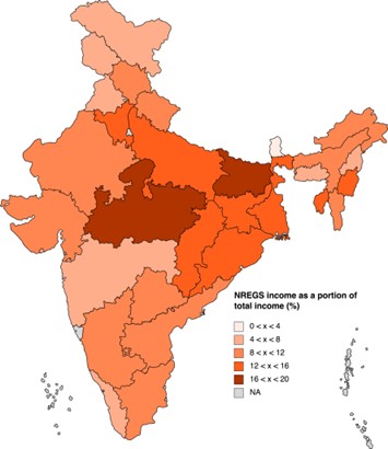
On a village level, current participation rates from NREGS appear to have a weak positive relationship on average household change in assets from 2005 to 2012. Figure 2 shows this relationship (non-participating villages removed), with the y-axis measuring the residuals from a linear regression of mean change in assets (assets in IHDS-II minus assets in IHDS-I) on mean consumption, education and non-NREGS income. The graph shows that higher household participation in a village is associated with higher average change in productive asset ownership over time, even after controlling for key socio-economic variables. More empirical work is needed to establish any causal impact from the scheme, since the aggregation of household data to a village level leaves this weak relationship susceptible to unknown sources of endogeneity.

Figure 2: Average change in productive assets and average NREGS income by village

IV. Methodology

I hypothesise that participation in the scheme will have a positive and statistically significant eﬀect on the ownership of productive household assets. There are two plausible causal mechanisms in which this relationship may exist. Firstly, an increase in employment availability may increase total household labour hours in a given year (assuming the NREGS isn’t used entirely as a substitute to other forms of employment), particularly during the agricultural oﬀ-season when little work is available in rural villages. This is expected to increase annual income, especially if the NREGS wage is higher than other forms of casual work in rural India. Assuming the marginal propensity to consume isn’t equal to one, this additional income will increase household savings (as shown in Ravi and Engler 2015). Consequently, households are more able to purchase assets that have high market values relative to ordinary consumer goods. Secondly, the NREGS oﬀers insurance against income shocks (Johnson, 2009), since it provides employment during the agricultural oﬀ- season and extreme weather events. The availability of employment may therefore act as a preferred substitute to common coping strategies of poor households when experiencing an income shock, namely dissaving and asset liquidation. This assumes that NREGS work is easily available, a less plausible assumption given that only 3 in 10 households who want NREGS work actually participated.

To test this hypothesis, this study will estimate the eﬀect of participation in the NREGS using a diﬀerence- in-diﬀerence (DID) model, in line with most of the relevant empirical literature (Liu and Deininger, 2010; 2019; Berhane et al., 2014; Ravi and Engler, 2015; Bose, 2017; Varman and Kumar, 2020). The least specified model is expressed as:

$l o g (P A S S E T S_{h} t) = α + θ s + ß_{1} P A R T_{h} + ß_{2} P O S T_{t} + ß_{3} (P A R T_{h} * P O S T_{t}) + δ X_{h} + Ɛ_{h} s t$

Where PART is the treatment binary variable, POST is the time binary variable, and PASSETS is the outcome variable that measures productive household asset ownership. For full descriptions and summary statistics of all variables within the model, see Table B in the appendix. The key coeﬃcient of interest, β₃, is given as the diﬀerence in diﬀerences:

$ẞ_{3} = E (P A S S E T S_{1}^{T} - P A S S E T S_{0}^{T}) - E (P A S S E T S_{1}^{C} - P A S S E T S_{0}^{C})$

A selection of relevant control variables are included, represented by the X_h matrix. Household income, consumption and education variables are added to control for variation which isn’t determined by partici- pation but has an impact on household assets. They are included only as pre-implementation variables to

prevent multicollinearity between control variables and the treatment variable, which could lead to underes- timation of the average treatment eﬀect. In addition, state fixed eﬀects are added to the model to account for varying social norms and economic conditions across states that aﬀect overall levels of productive asset ownership as well as the speed, coverage and quality of the NREGS implementation. By including confound- ing variables, the participation variable is prevented from accounting for the eﬀects of characteristics that are associated with both a change in the probability of participation as well as a change in productive assets over time. This reduces the likelihood of omitted variable bias, leading to a more accurate estimate of the average treatment eﬀect.

Further specifications include the log transformation of the outcome variable (in order to obtain more inferable estimates), as well as the inclusion of a poor binary variable within a triple interaction term (in order to identify heterogeneous impacts). The most specified model is therefore given as:

$l o g (P A S S E T S_{h} t) = α + θ_{s} + ß_{1} P A R T_{h} + ß_{2} P O S T_{t} + ß_{3} P O O R_{ħ} + ß_{4} (P A R T_{h} * P O S T_{t}) + ß_{5} (P A R T_{h} * P O S T_{t} * P O O R_{h}) + δ X_{h} + Ɛ_{h} s t$

Where β₅ is the diﬀerence in eﬀect between poor and non-poor households. As with all programmes that are based upon voluntary participation, self-selection is a problem, since the characteristics of households in each group diﬀer (see Table 1). If this isn’t accounted for, diﬀerences in outcomes between participants and non-participants that derive from diﬀerent levels and trends of pre-NREGS characteristics will be represented through the participation variable. Consequently, the estimated average treatment eﬀect will be biased and causal impacts will not be identified.

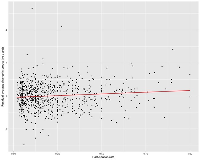
Therefore, a crucial part of the empirical strategy within this paper is to establish plausible counterfactuals as a control group. A simple and eﬀective way to do this is to establish control households as those that did not participate in the scheme but applied to work on the scheme (hold a job card). Since implementation, the NREGS has failed to meet total demand for work and a significant proportion of applicants are rejected (see Figure 1(a) and Dutta et al., 2012). This introduces exogenous variation between the allocation of treatment and control. However, it is worth noting that selection for work may not be entirely random; Das (2015) shows that households which support the ruling state party are more likely to receive work on the scheme. Despite this, subsetting to job card holders evidently reduces diﬀerences between treatment and control groups pre-implementation. Figure 3 shows how the majority of key household variables are no longer statistically diﬀerent (as opposed to Table 1) at 95 percent confidence intervals, which means that diﬀerence in outcomes between the groups can be more plausibly attributed to participation in the NREGS. In total, there are 11,791 households with at least one job card in the dataset.

Figure 3: Standardised pretreatment variables (mean and 95% conf. intervals) of job card households, grouped by participation

Whilst establishing non-participating job card holders as the control group has significantly reduced the extent of selection bias within the model, the issue has not been entirely fixed. Pretreatment averages of productive assets are significantly higher for participating households compared to non-participating job card households. This is an issue, since baseline asset levels are negatively correlated (Pearson Product Moment coeﬃcient of -0.28) with the change in assets for the entire dataset, suggesting that participants would have a lower change in assets regardless of the NREGS being implemented. This suggests that the parallel trends assumption has not been met (although there is no data from another pre-implementation time point to check this) and consequently the DID would be downward biased without appropriate correction.

Given these conditions, a matching strategy has been adopted, where participant and non-participant job card holders are paired based on pretreatment levels of productive asset ownership. This strategy is advised in Ryan, Burgess and Dimick (2015) for DID estimation when two conditions are present: 1. There’s a statistical diﬀerence in pretreatment outcome levels of each group, and 2. There is a relationship between pretreatment outcome levels and expected change in outcome which is not due to the treatment itself. Whilst matching does result in a smaller sample, the benefit is that treatment and control groups are more similar in terms of baseline asset holdings, which helps to make the parallel trends assumption more plausible. All treatment observations are included, each matched to one control observation. Matching is one-to-one and exact, given the discrete nature of the outcome variable. This avoids the pitfalls of information loss when using multivariate propensity score matching, as highlighted in King and Nielsen’s influential 2019 article.

One weakness of this approach derives from the aggregated nature of the outcome variable; observations with the same total productive asset levels will be matched despite these households owning diﬀerent types of assets. For example, one household that owns mainly utilities and appliances can be matched to another household which owns mainly livestock, technological items or a vehicle. This is a problem since diﬀerent assets provide households with diﬀerent capabilities to accumulate more assets. Therefore, one assumption required for the matching strategy to impose parallel trends is that asset compositions for treated and control observations have similar categorical distributions.

Another concern is the lack of pretreatment outcomes from multiple time points. Research by Chabé-Ferret (2017), which tested the performance of matching on pretreatment outcomes using simulations and revisiting past empirical studies, found that this matching strategy doesn’t perform as well when only one pretreatment time point exists, and in some cases is capable of actually increasing the DID bias. This research opposes the conclusions made by Ryan, Burgess and Dimick (2015). Given the mixed evidence on the eﬀectiveness of pretreatment outcome matching, the results will include both unadjusted and matched data, as recommended by Lindner and McConnell (2019).

Whilst a plausible strategy for mitigating selection bias has been adopted (subsetting to job card holders, controlling for confounding variables and matching on pretreatment asset holdings), the spillover eﬀects of the NREGS are unaccounted for. There is an abundance of empirical evidence which establishes a positive causal eﬀect of the implementation of NREGS on rural labour market wages. Berg et al. (2018) found that implementation caused growth in agricultural wages to increase by 4.3 percent, whilst Imbert and Papp (2015) find the average level eﬀect on casual labour wages to be 4.7 percent. As a result of the increased labour demand from the NREGS, the private sector experienced a crowding out eﬀect and remaining labourers had increased bargaining power in wage negotiations. This led to higher equilibrium wages for non-participants, who may have accumulated more assets as a result, despite not being directly involved in the NREGS. Therefore, the DID coeﬃcient is likely to be an underestimation of the scheme’s real impact (compared to the scenario in which the scheme was never administered). Of course, this assumes that wage gains made by non-participants weren’t cancelled out by a proportionate inflationary eﬀect in sectors that compete with the NREGS for labour, which may have kept real wages and disposable income constant.

V. Results

Breusch-Pagan tests were used to detect non-constant variation of the residuals in all of the models. Con- sequently, heteroskedasticity-consistent standard errors were adopted to restore confidence in the significance tests. Linear regression results for unadjusted and matched households are shown in Table 2.

Table 2: Log-level diﬀ-in-diﬀ regressions on total productive asset ownership using robust standard errors

	Unadjusted	Unadjusted	Matched	Matched
Intercept	1.685*** (0.118)	1.750*** (0.118)	1.779*** (0.131)	1.838*** (0.130)
PART	-0.019** (0.007)	-0.026** (0.008)	-0.032*** (0.009)	-0.032** (0.010)
POST	0.269*** (0.005)	0.253*** (0.006)	0.244*** (0.008)	0.228*** (0.009)
POOR			-0.118*** (0.008)	-0.114*** (0.013)
XINC	0.007*** (0.000)	0.007*** (0.000)	0.006*** (0.000)	0.006*** (0.000)
XCONS	0.009*** (0.000)	0.008*** (0.000)	0.007*** (0.000)	0.006*** (0.001)
XEDUC	0.024*** (0.001)	0.023*** (0.001)	0.020*** (0.001)	0.020*** (0.001)
PART:POST	0.022* (0.010)	0.030** (0.012)	0.047*** (0.011)	0.055*** (0.013)
PART:POST:POOR			-0.026 (0.021)	-0.036 (0.025)
R²	0.400	0.408	0.440	0.447
Adj. R²	0.399	0.407	0.438	0.446
Obs	23580	23580	12867	12867

***p < 0.001; **p < 0.01; *p < 0.05

In the unadjusted regression, participation in the scheme is associated with a 2.2 percent increase in productive asset ownership from 2005 to 2012 compared to non-participants, significant at the 5 percent level. This estimate increases to 4.7 percent and becomes more significant for the one-to-one matched dataset. This increase was expected, given that matching eliminated the higher average pretreatment asset count for participants which was negatively correlated with the change in assets in the full dataset. Although they are diﬀerent between unadjusted and matched models, these estimates both show a small but significant average eﬀect of the scheme, indicating low model dependence for this specific relationship. All household control variables are statistically significant and have a positive impact. Overall, the models account for between 40-45 percent of the total variation in productive asset ownership across households and time, with the R-Squared higher for the matched data.

Combining the double and triple interaction terms, we see that the average treatment eﬀect for poor households is 0.4 and 1.9 percent in each model, although the estimates are not significant. This represents a negligible impact for households below the poverty line, particularly when considering the extended time frame of 7 years.

Table 3: Log-level matched diﬀ-in-diﬀ regressions on asset outcomes using robust standard errors

	Technological items	Utilities & appliances	Vehicle	Livestock
(Intercept)	0.120 (0.098)	1.533*** (0.161)	0.864*** (0.177)	-0.189 (0.354)
PART	-0.015* (0.008)	-0.017 (0.013)	-0.060*** (0.014)	0.031 (0.028)
POST	0.493*** (0.007)	0.186*** (0.011)	-0.001 (0.012)	-0.147*** (0.025)
POOR	0.011 (0.010)	-0.104*** (0.016)	-0.084*** (0.018)	-0.019 (0.036)
XINC	0.003*** (0.000)	0.008*** (0.001)	0.002** (0.001)	0.005** (0.001)
XCONS	0.004*** (0.000)	0.004*** (0.001)	0.003** (0.001)	0.018** (0.001)
XEDUC	0.006*** (0.001)	0.023*** (0.001)	0.010*** (0.001)	0.000 (0.002)
State binaries	Variable	Variable	Variable	Variable
PART:POST	0.026** (0.010)	0.036* (0.016)	0.043* (0.018)	0.055 (0.036)
PART:POST:POOR	-0.039* (0.019)	-0.005 (0.031)	-0.018 (0.034)	-0.113 (0.068)
R²	0.565	0.548	0.265	0.108
Adj. R²	0.563	0.546	0.263	0.106
Observations	12858	12858	12858	12858

***p < 0.001; **p < 0.01; *p < 0.05

Table 3 shows the fully specified model with the outcome variable separated into individual assets and asset groups. From 2005 to 2012, participation in the NREGS is associated with a 4.3 percent increased probability of owning a vehicle for non-poor households. This probability falls to just 2.5 percent for poor households (although statistically insignificant). Positive and significant eﬀects on non-poor households also exist for technological items (2.6 percent) as well as utilities and appliances (3.6 percent), where technological items is the only asset class where the NREGS had a statistically diﬀerent eﬀect for poor households. Whilst insignificant, the DID estimate for livestock ownership is the largest for the non-poor out of all the asset outcomes, at 5.5 percent, with a relatively large but insignificant heterogeneous eﬀect as well (11.3 percent).

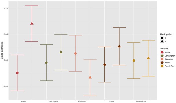
Figure 4: Heterogenous accumulation eﬀects of participation in the NREGS

Figure 4 shows the estimated treatment eﬀects and standard errors of participation in the NREGS for poor and non-poor households. From inspection, we can see that poor households only experienced positive eﬀects statistically diﬀerent from zero for utilities and appliances. All other asset classes and the total ownership variable had insignificant eﬀects for the poor. In contrast, non-poor households experienced positive and significant eﬀects for all asset classes. Statistically heterogenous eﬀects exist for technological items and livestock as well as the total productive asset ownership treatment eﬀect.

VI. Discussion and Conclusion

Overall, results from the model show mostly positive but mixed eﬀects of India’s National Rural Employ- ment Guarantee Scheme on productive asset accumulation. Matched data reveals the nationally represen- tative DID estimate to be 4.7 percent from 2005 to 2012, significant at the 0.1 percent level. Although this average eﬀect is not large, it is still economically significant in that it shows the scheme has enabled households to plan ahead and gradually accumulate physical productive assets over time. Furthermore, the average treatment eﬀect is likely to be larger than estimated due to the presence of spillover bias which was unaccounted for, as mentioned in the methodology section.

Whilst the results confirm the positive impacts of the scheme found by Deininger and Liu in 2019, they tell a diﬀerent story in terms of magnitude and heterogeneity. Their research found a 16.4 percent DID estimate on non-financial assets over just two years in Andhra Pradesh, an eﬀect over three times the size during a time interval less than half the length. To an extent this was expected, given that Andhra Pradesh was relatively successful (and received more funding per capita) in terms of NREGS implementation compared to most other states, which would have increased employment security and capacity to save/accumulate. Nevertheless, my research shows that the NREGS has not been as impactful as suggested by results of previous state-specific studies.

Perhaps the most surprising finding, and where my results contradict Deininger and Liu’s the most, is that poor households experienced mixed and mostly insignificant treatment eﬀects. In all specifications, being a poor household was associated with a lower DID estimate than non-poor households, with the eﬀect on total productive asset ownership being smaller (1.9 percent) and not statistically diﬀerent from zero. This is concerning given that the NREGS was designed to benefit this specific group the most. Evidently, the NREGS has had a future poverty prevention eﬀect for non-poor households, who have built resilience to future risk and potential income shocks, but has not exhibited a poverty alleviation eﬀect on currently poor households by means of asset accumulation.

One possible explanation for the heterogeneous impact of the scheme is that, proportionately, the poor allocate more income towards consumption and servicing debt. Consequently, they have lower marginal propensities to save (Dynan, Skinner and Zeldes, 2004), which constrains their ability to purchase expensive goods which require saving. Whilst Ravi and Engler (2015) find that the probability to save increased by 21 percent for poor participating households, these increased holdings have not translated into increased asset ownership. Based on these joint findings, I hypothesise two reasons as to why the NREGS has increased the probability to save but hasn’t increased asset accumulation for the poor. Firstly, the scheme serves as employment insurance, and therefore the poor may have less incentive to save for income-generating assets such as livestock, since the NREGS may be a preferred substitute. Secondly, the unfortunate reality of job rationing on the scheme may have hindered the poor from planning and committing to long term saving targets, since the additional employment is not secure, reliable or guaranteed for most job card holders.

On a broader note, these results may suggest that behavioural and/or structural constraints exist which disproportionately aﬀect poor households’ capacity to accumulate assets in rural India. Empirical evidence by Nashold (2012) supports this notion (and my findings) of asset accumulation, concluding that “economic stasis” exists for the poor in this geographical context (p. 2041). Recent work by Balboni et al. (2021), which evaluates the impact of a randomised asset transfer scheme over 11 years in rural Bangladesh, is also consistent with my results. These studies provide evidence towards the existence of a poverty trap in rural South Asia, whereby separate equilibria exist, determined by the split accumulation paths that are segregated by a dynamic asset poverty threshold, as theorised by Carter and Barrett (2006).

This paper provides further evidence of the mixed outcomes of India’s National Rural Employment Guar- antee Scheme, which has caused modest productive asset accumulation for non-poor households and has had mostly insignificant eﬀects on the poor. Findings from matched and unadjusted diﬀerence-in-diﬀerence models reinforce the results from existing research on the impacts of workfare on asset accumulation by Berhane et al. (2014), Ravi and Engler (2015) and Deininger and Liu (2019) and oﬀers new insight regarding heterogeneity of the average treatment eﬀect, consistent with the findings of Nashold (2012) and Balboni et al. (2021). Further research should investigate the potential factors that contribute to low relative ac- cumlation rates of poor participants, particularly vulnerability and job security, in order to identify specific improvements which can be made to optimise workfare policy as a mechanism for long term poverty reduction through asset accumulation. This research should take the changing context of the NREGS into account, which has been allocated additional funding since the COVID-19 pandemic to provide for the tens of millions of workers who have migrated back to their rural homes (Lokhande and Gundimeda, 2021).

VII. References

[1] Alik-Lagrange, and Ravallion, M. (2018). Workfare versus transfers in rural India’, World Develop- ment, 112, pp.244-258. Available at: https://doi.org/10.1016/j.worlddev.2018.08.008

[2] Azam, M. (2011). The impact of Indian job guarantee scheme on labor market outcomes: Evidence from a natural experiment’, Available at: https://dx.doi.org/10.2139/ssrn.1941959

[3] Bagchee, S. (1984). Employment Guarantee Scheme in Maharashtra’. Economic and Political Weekly 19, no. 37: 1633–38. http://www.jstor.org/stable/4373575.

[4] Balboni, , Bandiera, O., Burgess, R., Ghatak, M. and Heil, A., (2022). Why do people stay poor?’. The Quarterly Journal of Economics, 137(2), pp.785-844. Available at: https://doi.org/10.1093/qje/qjab045

[5] Banerjee, A. and Mullainathan, S. (2008). Limited attention and income distribution’. American Eco- nomic Review, 98(2), pp.489-93. DOI: 10.1257/aer.98.2.489

[6] Berg, , Bhattacharyya, S., Rajasekhar, D. and Manjula, R. (2018). Can public works increase equilib- rium wages? Evidence from India’s National Rural Employment Guarantee’. World Development, 103, pp.239-254. Available at: https://doi.org/10.1016/j.worlddev.2017.10.027

[7] Berhane, G., Gilligan, D., Hoddinott, J., Kumar, N. and Taﬀesse, A. (2014). Can social protection work in Africa? The impact of Ethiopia’s productive safety net programme’. Economic Development and Cultural Change, 63(1), pp.1-26. Available at: https://doi.org/10.1086/677753

[8] Besley, T. and Coate, S. (1992). Workfare versus welfare: Incentive arguments for work requirements in poverty-alleviation programs’. The American Economic Review, 82(1), pp.249-261. Available at: https://jstor.org/stable/2117613

[9] Bose, (2017). Raising consumption through India’s national rural employment guarantee scheme’.
World Development, 96, pp.245-263. Available at: https://doi.org/10.1016/j.worlddev.2017.03.010

[10] Carter, and Barrett, C. (2006). The economics of poverty traps and persistent poverty: An asset-based approach’. The Journal of Development Studies, 42(2), pp.178-199. Available at: https://doi.org/10.1080/00220380500405261

[11] Chabé-Ferret, (2017). Should we combine diﬀerence in diﬀerences with conditioning on pre-treatment outcomes?’. Université Toulouse 1 Capitole. Available at: http://tse-fr.eu/pub/31798

[12] Das, (2015). Does political activism and aﬃliation aﬀect allocation of benefits in the rural employment guarantee program: Evidence from West Bengal, India’. World Development, 67, pp.202-217. Available at: https://doi.org/10.1016/j.worlddev.2014.10.009

[13] Deaton, A. (1989). Saving in developing countries: Theory and review’. The World Bank Economic Review, Vol. 3(suppl_1), pp.61-96. Available at: https://doi.org/10.1093/wber/3.suppl_1.61

[14] Deininger, and Liu, Y. (2019). Heterogeneous welfare impacts of national rural employment guarantee scheme: Evidence from Andhra Pradesh, India’. World Development, 117, pp.98-111. Available at: https://doi.org/10.1016/j.worlddev.2018.12.014

[15] Desai, S., Vanneman, R., and National Council of Applied Economic Research. (2005). India Human Development Survey (IHDS). Inter-university Consortium for Political and Social Research [distributor], 2018-08-08. https://doi.org/10.3886/ICPSR22626.v12

[16] Desai, , and Vanneman, R. (2012). India Human Development Survey II (IHDS-II). Inter-university Consortium for Political and Social Research [distributor], 2018-08-08. https://doi.org/10.3886/ICPSR36151.v6

[17] Dreze, and Sen, A. (1990). Hunger and public action. Clarendon Press.

[18] Dutta, , Murgai, R., Ravallion, M. and Van de Walle, D. (2012). Does India’s employment guarantee scheme guarantee employment?’. Economic and Political Weekly, pp.55-64. Available at: https://www.jstor.org/stable/23214599

[19] Dynan, K., Skinner, J. and Zeldes, S., (2004). Do the rich save more?’. Journal of political economy, 112(2), 397-444. Available at: https://doi.org/10.1086/381475

[20] Ehmke, E. (2015). National experiences in building social protection floors: India’s Mahatma Gandhi National Rural Employment Guarantee Scheme’. International Labour Organization. Available at: https://ideas.repec.org/p/ilo/ilowps/994884383402676.html

[21] Esteves, T., Rao, K., Sinha, B., Roy, S., Rao, B., Jha, S., Singh, A., Vishal, P., Nitasha, S., Rao, S. and IK, (2013). Agricultural and livelihood vulnerability reduction through the MGNREGA’. Economic and Political Weekly, pp.94-103.

[22] Fetzer, T., (2020). Can workfare programs moderate conflict? Evidence from India’. Journal of the European Economic Association, 18(6), pp.3337-3375. Available at: https://doi.org/10.1093/jeea/jvz062

[23] Gentilini, U., Almenfi, M., Iyengar, T., Okamura, Y., Downes, J., Dale, P., Weber, M., Newhouse, D., Rodriguez Alas, C., Kamran, M. and Mujica Canas, I., (2022). Social protection and jobs responses to COVID-19’. World Bank Group. Available at: http://hdl.handle.net/10986/37186

[24] Haque, (2011). Socio-economic Impact of Implementation of Mahatma Gandhi National Rural Employment Guarantee Act in India’. Social Change, 41(3), pp.445-471. Available at: https://doi.org/10.1177/004908571104100307

[25] Imbert, and Papp, J. (2011). Estimating leakages in India’s employment guarantee us- ing household survey data’. Paris School of Economics and Princeton University. Available at: http://riceinstitute.org/wordpress/wp-content/uploads/downloads/2012/02/ImbertPapp.pdf

[26] Imbert, C. and Papp, J. (2015). Labor market eﬀects of social programs: Evidence from india’s em- ployment guarantee’. American Economic Journal: Applied Economics, 7(2), pp.233-63. Available at: https://aeaweb.org/articles?id=10.1257/app.20130401

[27] Johnson, (2009). Can workfare serve as a substitute for weather insurance? The case of NREGA in Andhra Pradesh’. The Case of NREGA in Andhra Pradesh. Available at: http://dx.doi.org/10.2139/ssrn.1664160

[28] King, G. and Nielsen, R. (2019). Why propensity scores should not be used for matching’. Political Analysis, 27(4), pp.435-454. Available at: https://doi.org/10.1017/pan.2019.11

[29] Klonner, and Oldiges, C. (2022). The welfare eﬀects of India’s rural employment guarantee’. Journal of Development Economics. Available at: https://doi.org/10.1016/j.jdeveco.2022.102848

[30] Kundu, A. and Talukdar, S. (2016). Asset creation through National Rural Employment Guarantee Scheme (NREGS) and its impact on West Bengal agriculture: A district level analysis’. Journal of Global Economy, 12(3). Available at: https://ssrn.com/abstract=2844656

[31] Lindner, and McConnell, K.J. (2019). Diﬀerence-in-diﬀerences and matching on outcomes: a tale of two unobservables’. Health Services and Outcomes Research Methodology, 19(2), pp.127-144. Available at: https://link.springer.com/article/10.1007/s10742-018-0189-0

[32] Liu, and Deininger, K.W. (2010). Poverty impacts of India’s national rural employ- ment guarantee scheme: Evidence from Andhra Pradesh’. (No. 320-2016-10232). Available at: https://ideas.repec.org/p/ags/aaea10/62185.html

[33] Lokhande, and Gundimeda, H. (2021). MGNREGA: The Guaranteed Refuge for Returning Migrants During COVID-19 Lockdown in India’. The Indian Economic Journal, 69(3), pp.584-590. Available at: https://doi.org/10.1177/00194662211023848

[34] Ministry of Rural Development. (2013). MGNREGA operational guidelines, 4th edition. Available at: https://nrega.nic.in/Circular_Archive/archive/Operational_guidelines_4thEdition_eng_2013.pdf

[35] Morduch, (1999). Between the state and the market: Can informal insurance patch the safety net?’. The World Bank Research Observer, 14(2), pp.187-207. Available at: https://doi.org/10.1093/wbro/14.2.187

[36] Naschold, (2012). The poor stay poor: Household asset poverty traps in rural semi-arid India’. World Development, 40(10), pp.2033-2043. Available at: https://doi.org/10.1016/j.worlddev.2012.05.006

[37] Naudé, , Santos-Paulino, A. and McGillivray, M. (2009). Measuring vulnerability: An overview and introduction’. Oxford Development Studies, 37(3), pp.183-191. Available at: https://doi.org/10.1080/13600810903085792

[38] Nayak, (2013). Determinants and pattern of saving behavior in the rural households of western odisha’ (Doctoral dissertation). National Institute of Technology. Available at: http://ethesis.nitrkl.ac.in/4839/

[39] Peck, (1998). Workfare: a geopolitical etymology’. Environment and Planning D: Society and Space, 16(2), pp.133-161. Available at: https://doi.org/10.1068/d160133

[40] Ranaware, , Das, U., Kulkarni, A. and Narayanan, S. (2015). MGNREGA works and their impacts: A study of Maharashtra’. Economic and Political Weekly, pp.53-61. Available at: https://www.jstor.org/stable/24481747

[41] Ravallion, (1991). Reaching the rural poor through public employment: arguments, evidence, and lessons from South Asia’. The World Bank Research Observer, 6(2), pp.153-175. Available at: https://doi.org/10.1093/wbro/6.2.153

[42] Ravi, and Engler, M. (2015). Workfare as an eﬀective way to fight poverty: The case of India’s NREGS’. World Development, 67, pp.57-71. Available at: https://doi.org/10.1016/j.worlddev.2014.09.029

[43] Reddy, A., Roy, N. and Pradeep, D. (2021) ‘Has India’s Employment Guarantee Program Achieved Intended Targets?’, SAGE Open. Available at: https://doi.org/10.1177/21582440211052281

[44] Ryan, , Burgess Jr, J. and Dimick, J. (2015). Why we should not be indiﬀerent to specifica- tion choices for diﬀerence-in-diﬀerences’. Health services research, 50(4), pp.1211-1235. Available at: https://doi.org/10.1111/1475-6773.12270

[45] Sen, A. (2006). Conceptualizing and measuring poverty’. Grusky, D., Kanbur, R. (EDS.). Poverty and Inequality, Stanford, California: Stanford University Press. pp.30-46.

[46] United Nations Department of Economic and Social Aﬀairs. (2021). End Poverty in All its Forms Ev- erywhere. Available at: https://sdgs.un.org/goals/goal1 (accessed April 25th 2022).

[47] Varman, P.M. and Kumar, N., (2020). Impact of MGNREGA on Consumption Expenditure of House- holds’. Economic & Political Weekly, 55(39), p.49.

[48] Vatsa, K. (2004), Risk, vulnerability, and asset-based approach to disaster risk management’, In- ternational Journal of Sociology and Social Policy, Vol. 24 No. 10/11, pp. 1-48. Available at: https://doi.org/10.1108/01443330410791055

[49] Walker, , Singh, R. and Asokan, M. (1986). Risk benefits, crop insurance, and dryland agriculture’.
Economic and Political Weekly, pp.A81-A88. Available at: https://www.jstor.org/stable/4375827

[50] Zimmermann, (2012). Labor market impacts of a large-scale public works program: evidence from the Indian Employment Guarantee Scheme’. IZA Discussion Paper No. 6858. Available at: https://papers.ssrn.com/sol3/papers.cfm?abstract_id=2158000

Appendix

Table A: Data sources and credits

Data source	Download link	Website	Principal Investigators
IHDS-I	https://www.icpsr.umich.edu/web/DSDR/studies/22626	https://ihds.umd.edu/	Sonalde Desai, University of Maryland;
IHDS-II	https://www.icpsr.umich.edu/web/DSDR/studies/36151	National Council of Applied Economic Research, New Delhi	Reeve Vanneman, University of Maryland;

Table B: Description and summary of key variables

Variable Name	Description	Mean	Std. Dev	Min	Max
PASSETS	Sum of binary ownership variables, representing the total number of diﬀerent productive assets the HH owns	5.47	2.71	0.00	15.00
POST	Binary time variable which equals one when the observation is from the second IHDS	0.50	0.50	0.00	1.00
NWKNREGA	Discrete variable where each unit represents one member of the HH with at least 240 hours working on the NREGS in the past year	0.10	0.38	0.00	6.00
IN16	Discrete variable where each unit represents one member of HH with a job card for the NREGS	0.33	0.54	0.00	5.00
INCNREGA	Continuous variable which represents the total HH income earned through the NREGS (000 Rs)	0.89	2.90	0.00	100.00
PART	Binary variable which equals one when NWKNREGA > 0	0.08	0.27	0.00	1.00
POOR	Binary variable which equals one when total HH income < poverty line	0.23	0.42	0.00	1.00
XINC	Total HH income in 2004/2005 (000 Rs)	98.78	148.72	-429.75	12032.85
XCONS	Total HH consumption expenditure in 2004/2005 (000 Rs)	100.10	95.42	0.69	1901.77
XEDUC	Highest years of education of any HH member at least 21 years old (IHDS1)	7.43	5.01	0.00	15.00

Note: Statistics derive from 39,857 complete observations in the dataset